Valve pressure drop test

About the author

Chao-Sheng Chen is the General Manager of Kong Jih Valve Ind. Co., Ltd., an established Taiwanese valve manufacturer. Together with Chin-Chi Chang of the engineering department, they have benchmarked AirShaper against both their internal calculations and physical test results.

Ball valves

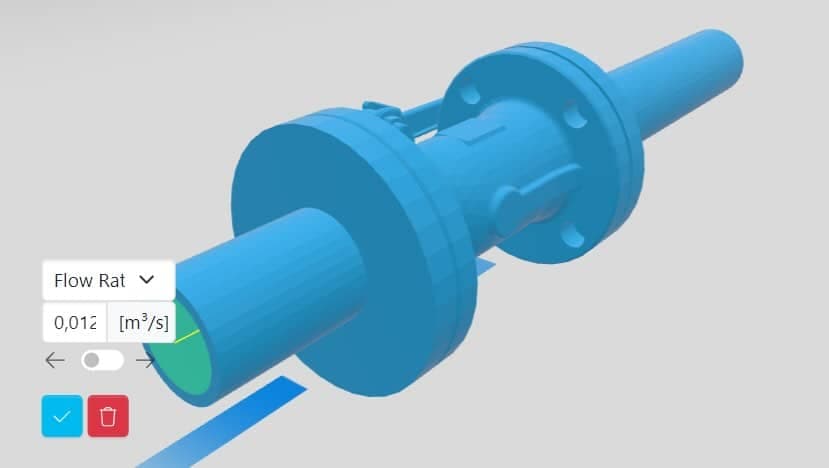
A ball valve is a popular fluid-control device -- it is durable and easy to repair. But a valve also introduces resistance (in the form of a pressure drop), which increases the required energy to pump a fluid through the valve. The efficiency of a valve is indicated by the Flow Coefficient (Cv):

This Cv can thus be used to calculate the flow rate (given a certain pressure drop) or the pressure drop (given a certain flow rate). As this impacts the required energy, pumps, ... for fluid systems, customers are increasingly interested in obtaining accurate Cv values as input for their engineering teams.

Physical testing

The most direct approach to obtain Cv values is to perform a physical test, i.e. integrating the valve into a test system where the flow parameters (pressure upstream & downstream, flow rate) can be monitored. Based on the output, the Cv value can then be calculated. But this testing process is lengthy and costly. In addition, each design change requires a new test.

Approximate formulae

We have in-house formulae to predict the Cv values, but they are one-dimensional calculations. They don't take the geometrical details and complex flow aspects, i.e. boundary layers, flow separation, etc., into account. They are relevant to obtain the right order of magnitude, but not precise enough to replace a test. For example, for the valves tested in this study, we observed deviations up to 68% between the calculated values and the physical test results. Using these, we'd have to add a large uncertainty margin, ending up with conservative Cv values for our customers.

CFD simulations

To obtain more precise Cv values without having to test each design, we turned to AirShaper for their simulation expertise. To gain confidence, we provided AirShaper with the test data of 2 different valves at various flow rates. We wanted to know the influence of different parameters on the Cv values, so that we could select the right setup for us to analyze other valves in the future.

Valves types

We analyzed two valve types for this benchmark.

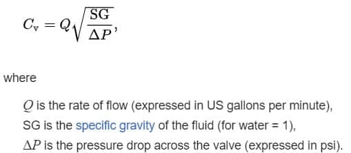
• Sample A -- straight flow passage: this valve features very little obstruction on the inside. As such, the flow resistance is mainly determined by what happens in the boundary layer.

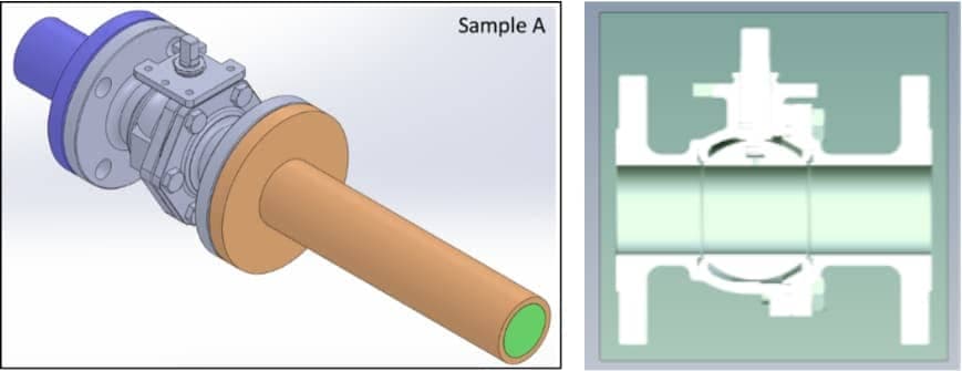
• Sample B -- non-straight flow passage: this valve features a contraction as well as a more pronounced obstruction of the flow. As such, the flow resistance will be higher and more dependent on flow separation around these geometries.

CFD -- computational fluid dynamics

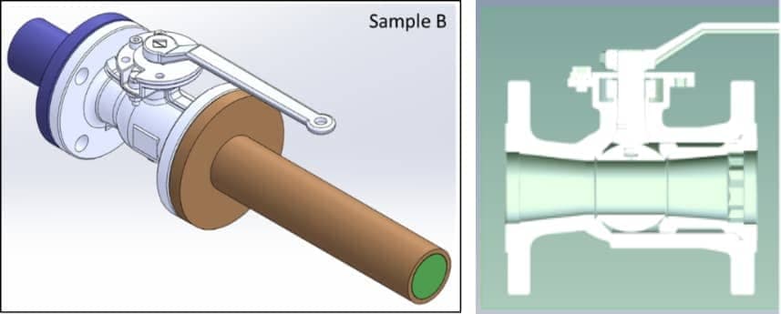
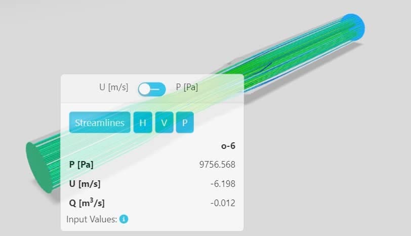
We added upstream & downstream pipes to allow the velocity profile to develop before & after the valve. The pressure measurements were performed at the start & end of these additional pipes. We added a flow rate constraint at the inlet, and a 0-pressure constraint at the outlet.

The results included the flow rate & pressure drop across the entire system. This allowed the AirShaper software to calculate the pressure difference, which we needed to calculate the Cv values.

Parameter sensitivity

Layers

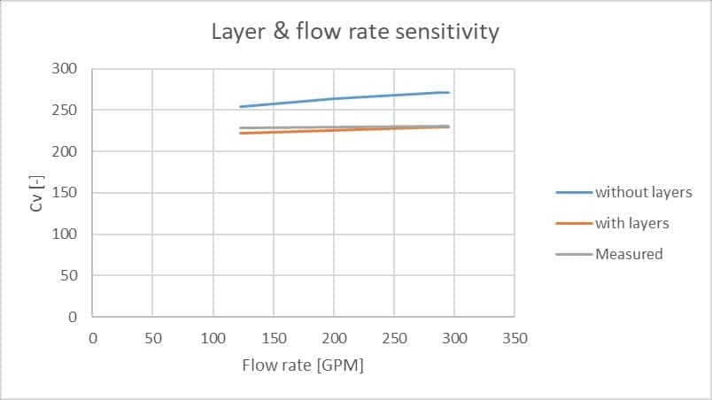
The addition of prism layers to the mesh provides a more realistic approach to capturing the boundary layer.

• Sample A: The addition of layers leads to a big improvement, reducing the variations between the test data and the simulation to just 0.9% at the highest flow rate.

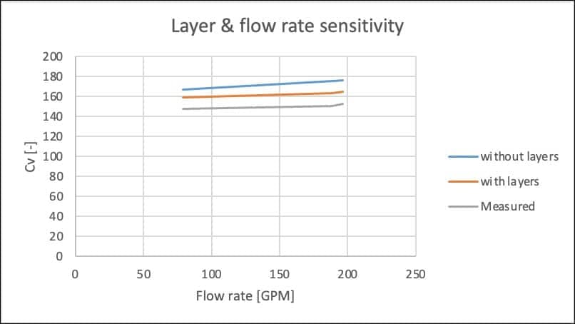
• Sample B: the addition of layers again had a positive effect, although less pronounced. This is expected, as the impact of the boundary layer is relatively low due to the geometrical obstructions.

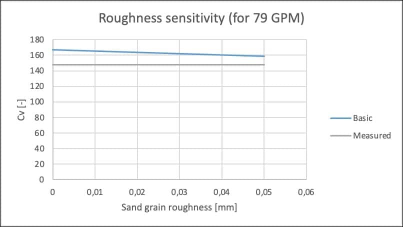
Surface roughness

Just like the prism layers, the surface roughness also impacts the boundary layer and the friction on the wall. Although the internal surface of the valve is quite smooth, we added roughness to see how strong the effect would be (the analyses were done for 1 flow rate only).

• Sample A: here too, sample A is quite affected by the roughness due to the relative importance of the boundary layer. Increasing the surface roughness by too much, lead to a larger variation again.

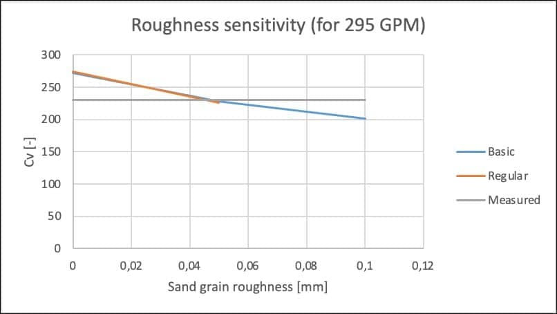
• Sample B: as expected, the impact of surface roughness is less pronounced:

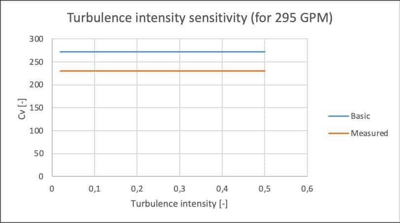
Turbulence intensity

The turbulence intensity at the inlet was increased, but no noticeable change in Cv was observed.

Conclusion

By studying the sensitivity of different parameters, we concluded that the Basic AirShaper simulations with layers, without roughness, were the best compromise to obtain reliable values for sample A and sample B. For sample A, this resulted in less than 1% deviation. For sample B, the deviation was around 10%.

In general, the simulated values are close to the actual test values. Although the deviation is slightly higher for sample B, this method is a far more accurate method than our one dimensional calculation tool. AirShaper has provided us with an efficient, accurate and economical way to obtain Cv values through simulation.