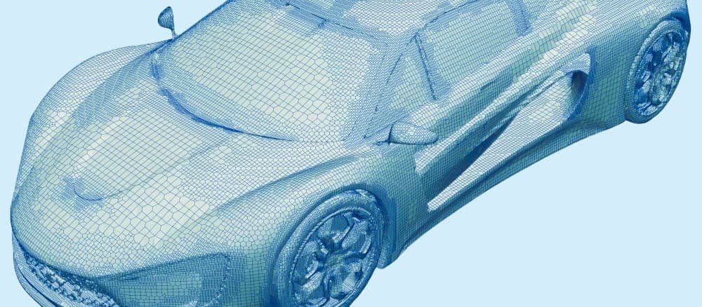
Multi-fidelity optimization of a fixed-wing drone using geometric Convolutional Neural Networks.
January 29, 2020
1 Introduction
Optimizing the shape of UAVs is of primary importance for the industry. SenseFly, one of the mar- ket leaders in the fixed-wing drone segment is always looking to minimize the battery consumption of its aircrafts and therefore offer longer flight ranges to its customers. Since the external design has a very direct and radical influence on in-flight performances, even a slight improvement is crucial and brings a non-negligible technological lead on the other actors. Numerical simulations can be used to assess the performance of the design on a range of flow velocities and flight conditions, without actually building the drone. Nevertheless, these simulations are numerically expensive and therefore multiple fidelities can be used. The AirShaper platform lets the engineer upload a 3D model (via the web interface or via the API service) to have the aerodynamics analyzed in the cloud. Even with a very efficient and reliable numerical simulator, manual optimization remains a tedious process. In this report, we show how the Neural Concept Shape optimization platform can be gracefully combined with AirShaper and exploit the multiple fidelities to reach an optimal design that achieves better flight performances.
2 Method Overview
2.1 Numerical optimization using Neural Concept Shape
Numerical simulations have become of primary importance for the industry over the last decades. Nevertheless, since a simulation must be re-run each time an engineer wishes to change the shape which is being designed, it makes the engineering process slow and costly. A typical approach is therefore to test only a few designs without a fine-grained search in the space of potential variations. This is a severe limitation and there have been many attempts at overcoming it and automating the shape optimization process, but none has been entirely successful yet. A classical approach to reduce the computational complexity is to use surrogate modelling via Gaussian Process (GP) regressors, or others, trained to interpolate the performance landscape given a low dimensional parametrization of the shape space. This interpolator is then used as a proxy for the true objec- tive to speed-up the computation, which is referred to as Kriging in the literature. However, those regressors are only effective for shape deformations that can be parameterized using relatively few parameters and their performance therefore hinges on a well-designed parameterization. Fur- thermore, the regressors are specific to a particular parameterization and pre-existing computed simulation data using different ones cannot be easily leveraged. A recently developed software, Neural Concept Shape (NCS), empowers the engineer with a new tool, Geometric Convolutional Neural Networks, to build surrogate models of numerical solvers. It suffers from none of the drawbacks of previous surrogate methods, such as the Kriging one. It is agnostic to the shape parameters as it processes directly the mesh representation of the design. Hence, optimization parameters are decoupled from the learning problem and a single predictor can be trained with a large amount of data and used for many optimization tasks. Unlike Kriging methods, the engineer does not have to choose and stick to a specific parametrization from the beginning to the end of experiments. Furthermore, it can leverage on transfer learning abilities of Deep Learning models to blend simulations from multiple sources and different parametrizations. To date, NCS is the only CAE-oriented Deep-Learning code that is able to process industrial scale raw unstructured 3D data directly, without any preprocessing. It uses multi-scale geometric neural networks, through a combination of surface such as geodesic and euclidean network architectures. It is able to learn to emulate simulators and reproduce multiple outputs such as integrated scalar values e.g. drag forces or energy consumption or surface and volumetric field values e.g. pressure or temperature.
2.2 Numerical Simulation with AirShaper
AirShaper (www.airshaper.com) is a cloud-based HPC (high-performance computing) platform for external aerodynamics. It automates the entire process to go from 3D model to a finished CFD (computational fluid dynamics) simulation. The required input is limited to the 3D file, the model scale, position & orientation. The output includes a pdf report with data (including drag & lift values) & flow visualizations, an online 3D viewer and the full flow field data in OpenFOAM format. The platform offers steady-state RANS simulations using the k-omega SST turbulence model, with automatic detection of convergence & sizing of the averaging window for consistent results. The platform is directly compatible with non-watertight 3D models (accepting gaps & holes) eliminating any CAD repair effort on the user side. An API (Application Programming Interface) is available to initiate & process simulations on AirShaper from within another software application. AirShaper has been awarded ”Motorsport Technology of the Year 2019” for its merits in the automotive segment.
2.3 Optimization approach
The aim of the project is to optimize the aerodynamic performance of one of SenseFly’s best- selling drones, while still satisfying aerodynamic and geometric constraints. We have access to three levels of accuracy for the simulator. The first level gives a very approximate estimate of the simulation results and corresponds to simulations generated by an internally set simulator. The second simulation level is the concept simulation from AirShaper, while the third simulation is the most accurate and corresponds to a detailed simulation from AirShaper. The detailed level of simulation is expensive to run and therefore we only have a budget of 50 such simulations, which is too small to efficiently optimize a design in our high-dimensional design space. The optimization framework within NCS lets us nevertheless pre-train a network with lower accuracy simulations, which is then fine-tuned with higher accuracy ones in order to do the final optimization at the most detailed level of simulation accuracy.

Denoting by Ω the set of feasible geometries the problem reads:
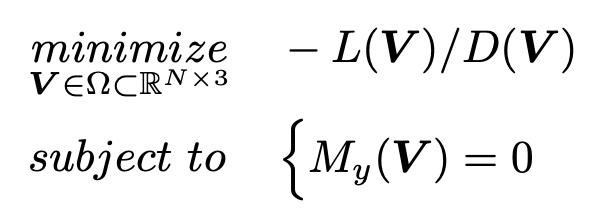
We are using the optimizer of Neural Concept Shape to set up an optimization loop between the Neural Network and the simulator where the simulator is called back automatically to generate new simulation samples that are then used to retrain the Neural Network using a specific internal strategy.
3 Setup in Neural Concept Shape
3.1 Optimization within NCS
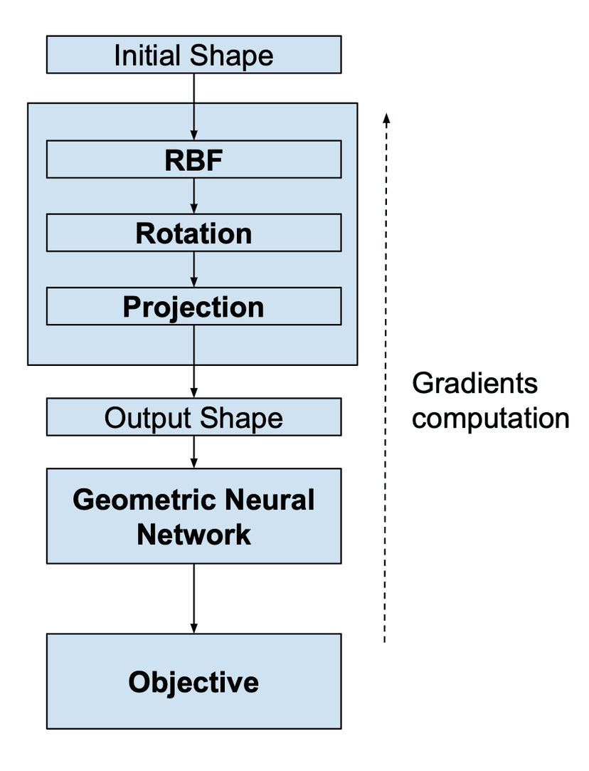
In order to reduce the number of optimization variables, to ensure a smooth deformation of the surface, and to handle the geometric constraints, a parametrization of the vertices V = P (V (0), z) is introduced. V(0) denotes the original vertices andzis a vector of the new design variables. The NCS framework lets the user define conveniently a set of parametrization modules that can be stacked to generate and optimize deformations with respect to an initial design.
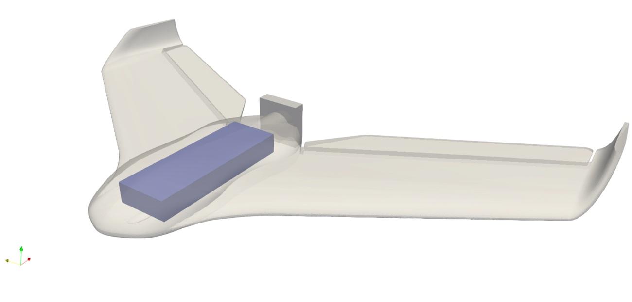
All the modules can be interchanged at any point of the optimization process. The shape constraints representing the electronics case which needs to be fitted inside the shape, can be defined also as a ”projection” parametrizer. The geometric constraints are shown with figure 6. The objective block lets the user define an objective function to optimize. The objective values given by the surrogate model and by the ground-truth are automatically stored and logged by the framework.
As described in Figure 4, the NCS framework lets us define all these components separately and connect them within the framework to perform the optimization, and in particular to propagate the derivatives for gradient-based optimization.
3.2 Parametrization
We define P(i)(z(i),V) as a continuous and differentiable transformation of the input vertices V, from SenseFly’s initial design, according to a variables vector z(i). Moreover we indicate as P(i)◦
P(j) the composition of two parametrization. We now report the three types of parametrization that we used:
- Radial Basis Function interpolation
- Projection
- Rotation
3.2.1 Radial Basis Functions
In order to smoothly deform the surface, we rely on the Radial Basis Function deformation of the shape. In this work, we use 50 control points that are chosen on the surface using a farthest point sampling heuristic. Every point is free to move in all three spatial directions and therefore we have 150 RBF optimization parameters. In Figure 5 we show the reference geometry (blue) and a random configuration where the 50 control points C(red) are randomly deformed with |Di,j| ≤ 0.02.

3.2.2 Projection
This parametrization is designed to ensure that the geometric constraints are satisfied at every iteration of the optimization process. The requirements impose to have a fuselage which is a rectangular cuboid of dimensions l = [Lx,Ly,LZ] = [220,75,30] [mm], see Figure 6. When a vertex enters the fuselage volume it needs to be projected back on its surface. The projection of the deformed vertices on the rectangular cuboid is done trough a linear map. Defining as y the deformed position of a vertex and as x its original position, the following must holds:
yi +(xi −yi)ti = sign(xi)li i = 1,2,3
Among the three candidates the one satisfying:
−l ≤ y + (x−y)ti ≤ l
is selected. We will denote this projection operation as P(proj)(V).
3.2.3 Rotation
Given an axiss, specified by two points p1 and p2 , and a rotation angle θ, the rotation of x0 aroundsis given as an additional parameter.
This parametrization is used to vary the angle of attack θ of the drone (a rotation around the y axis); however it could also be used to rotate some specific parts of the geometry, such as the elevators.
It adds one optimization parameter that corresponds to the rotation angle. Since the projector parametrization is stacked before the rotation, the constraint box ”rotates” with the angle of attack.
3.3 Geometric Neural Network
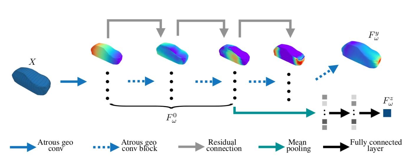
We use the typical ”PointRegressor” defined by the NCS framework as our Geometric Neural Network regressor. The architecture of our network is illustrated in 7. The first part of the model pre-processes the input and constructs a set of features by means of the previously introduced geodesic convolution operations. These features are then used to predict the global scalars via average pooling and two dense layers. The second branch of the network generates pressure fields relying on an additional set of geodesic convolutions and point-wise operations. The new network takes advantage of a GPU efficient implementation of geodesic convolutions, removing the need to use a Cube-Mesh mapping or any prior remeshing.
3.4 Objectives
In this project, the goal is to maximize the lift-to drag ratio of the drone, with a minimum value of lift to be guaranteed. NCS offers a module to directly define an optimization objective and constraints as a function of the output of the Neural Network prediction. The objective chosen corresponds to the target of maximizing the L/D and we add a numerical constraint to keep lift above a value of L= 8.0 [N].
4 Results
4.1 Pretraining optimization
As a first step, we run a full optimization against a low fidelity simulator. This optimization is used to start focusing the optimization on potentially interesting designs and to pre-train the Neural Network. In Figure 8 we show how the lift-to-drag ratio L/D (that we will call the objective) evolves over the iterations of the optimization process. Both the ground truth values and the predictions of the network are shown with their centered moving average (with a window sizen= 20). Moreover the relative error (and its moving average) are also shown.
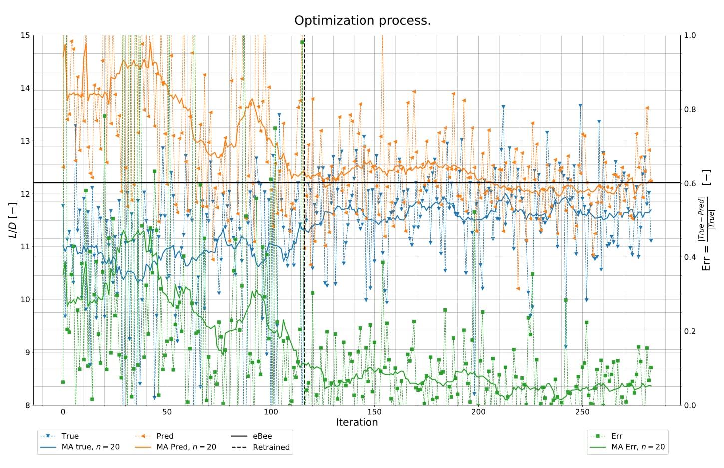
Figure 8 clearly shows that the mean objective value increases over time. The reference objective represents the maximum value of lift-to-drag ratio obtained by simulating the reference geometry for Nθ= 20 equi-spaced angles of attack − 2 ◦≤θ≤ 7 ◦. Even though the moving average is smaller than the reference objective, our interest is to find an increasing number of geometries better than the eBee.
4.2 Transfer learning
We now switch to the second phase of the optimization, where we aim at reusing the pre-trained network from 4 to initialize the surrogate model that will be used to optimize the design against the ”accurate” simulator from AirShaper. In Figure 9, we demonstrate the advantage of using a pre-trained network to initialize the second optimization phase. To show that, we compare the accuracy of the surrogate model trained from scratch on detailed simulations to the model pre-trained on the low-fidelity simulations and fine-tuned on the high-fidelity ones.
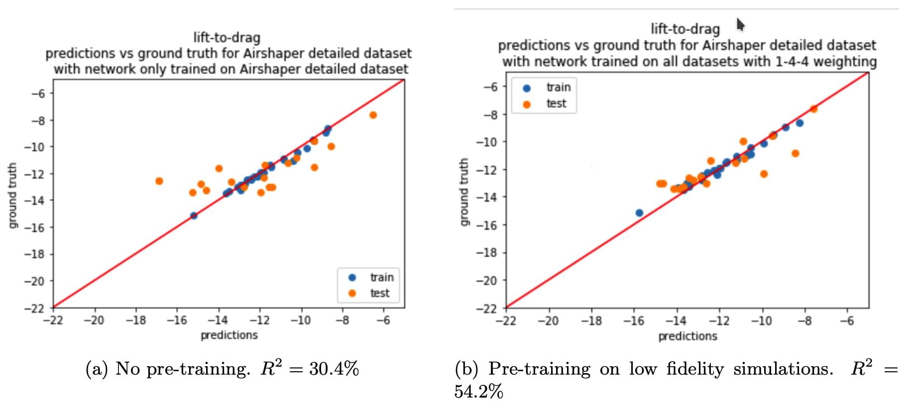
Figure 9: Predictions of L/D ratio on high-fidelity simulations for a model trained on high-fidelity simulations where: (a) The model was trained directly on 50 high-fidelity simulations. (b) The model was pre-trained before on low-fidelity ones. We can see that pre-training the network between fine-tuning it brings a substantial improvement (more than 20%) in R^2 error, which motivates the transfer-learning approach.
4.3 Final design
By comparing the original design to the optimized one, the lift to drag ratio has increased by 4.25% and the drag has been reduced by 6.25% at maximum L/D. It has to be noticed that the optimization process was run using only 40 detailed simulations and is already able to converge to much more efficient designs. It is interesting to see that the automatic optimization algorithm converges to some shapes & techniques that have been applied before in aviation. The result is a more organic shape, featuring:
- Anhedral wing setup: the wings of the optimized design feature a more pronounced anhedral setup (wings pointing downward). This will influence the pressure pattern on the wings and, although not included in the goal of this optimization, will also result in a more dynamic response of the drone (as opposed to the self-stabilizing effect of a dihedral wing setup wings pointing upward).
- Variable angle of attack: the angle of attack of the airfoil section of the wing changes across the length of the wings. In this case, the angle of attack increases towards the root of the wing, where there is interference with the flow around the fuselage.


- Winglet orientation: the winglets at the end of the wings, which are there to reduce the wingtip vortex, are tilted inward on the optimized design.


- Fuselage design: the fuselage in the optimized design features a more airfoil-like design, with a low leading edge and quite a lot of camber along the length (curvature of the main body). This helps to accelerate the airflow at the top of the fuselage, creating a low-pressure zone that generates additional lift on the body.

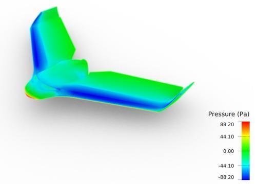
Figure 14: Pressure field displayed on the drone. The original design has a only slight camber on the fuselage.

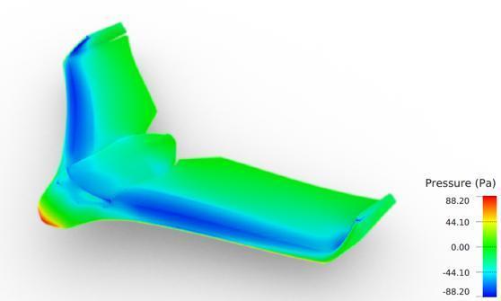
Figure 15: Pressure field displayed on the drone. The optimized design has a larger camber on the fuselage, generating additional lift.
Authors
We thank the authors and persons who have contributed to this paper:
Neural Concept: Juliette Marrie, Pierre Baque
AirShaper: Wouter Remmerie
EPFL: Francesco Bardi, Pascal Fua
Download Original Paper
