OpenFOAM Convergence detection

Problem statement

In addition to monitoring residuals, a common method to assess whether a simulation has converged is to look at the forces on an object. Especially for external aerodynamics, the drag, lift and lateral forces are usually of great interest (towards drag and lift coefficient, efficiency and power estimates, ...). It therefore makes sense to monitor these properties and wait until they are stable before starting the averaging.

OpenFOAM already provides such functionality through run-time control function objects. These allow, for example, to terminate the simulation as soon as the averaged drag coefficient is within a certain specified tolerance for a given number of steps. However, these parameters need to be determined manually for each case, making it difficult to use towards automation.

The open-source library presented here has been developed to provide fully automated convergence detection and averaging of OpenFOAM output data but is generally applicable to any data output for which convergence needs to be detected. It's been designed to automatically scale to the amplitude and length of the provided data, eliminating user input.

Suggested solution

Convergence detection

The theory behind the library is to mimic "human behaviour" to assess whether a curve has converged or not, following these steps:

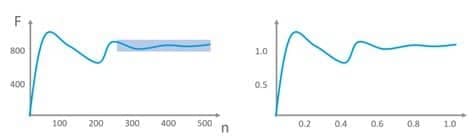
• Normalization When we evaluate a curve as a human, we do so looking at its proportions: how much does it oscillate versus the total height, for how long has the curve been flat versus the total length of the curve, etc. So we look at relative properties, which can mathematically be represented by normalizing the curve on both the horizontal axis (the number of iterations n) and the vertical axis (the force in this case, but this could be any parameter). In this library, we use the average force value of the last 50 percent of iterations (a window size of 0.5) to normalize the entire curve (and we do this again for each iteration). Fig. 1 illustrates this.

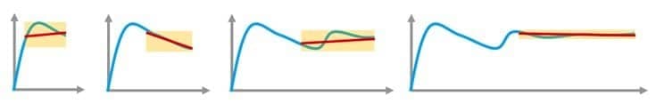
• Gradient calculation Once we have normalized the curve, we want to assess when the curve has "stabilized. That means that the last bit of the curve somehow needs to have been "stable enough" for "long enough". For each iteration, we fit a straight line through the last 50 percent (a window size of 0.5) of the normalized curve and store the gradient of this curve. Fig. 2 illustrates this.

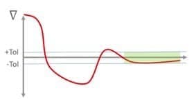
• Threshold This "running gradient" then indicates how stable the curve is (looking backwards) for each iteration. As we are working with a normalized curve, we can then define an absolute threshold value (irrespective of the magnitude of the force or the number of iterations) for this gradient to be within before we label a simulation as converged. We have chosen to evaluate this running gradient for the last third (so a window size of 0.33) of the curve. Fig. 3 illustrates this.

Averaging

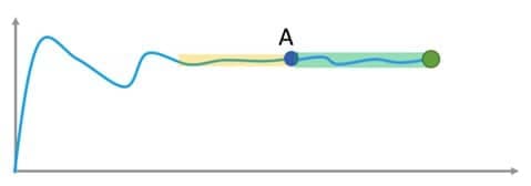
Dynamic window sizing - Once convergence has been detected, the simulation will start to average. A modified version of the conversion detection method will detect when the averaging has taken long enough to provide a reliable averaged value / reliable averaged fields -- see Fig. 4 (the yellow bar indicates the convergence detection, the green one the averaging window).

This detection method differs from the convergence detection method in the following ways:

• Normalization is frozen and the horizontal axis index will grow beyond 1. The longer a simulation runs, the lower the gradient value will become (as you divide by an ever-increasing index).

• The threshold values for the gradient are more strict (+-0.025 versus +-0.075).

• The evaluation window is now the entire length since the convergence point (versus a 0.5 window for the convergence detection), as there is no need any more to ignore initial oscillations. The whole averaging window needs to feature a stable curve.

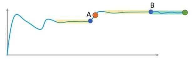
Re-start - In the background, this convergence detection method keeps running: sometimes, after convergence has been detected, the curve can go up or down and the gradient can "exit" the threshold band again. Fig. 5 illustrates how at point A the curve seemed to have converged (looking back at a flat part) but then suddenly rose (see the orange dot). In that case, the state of the simulation will again be set to "not converged" until the convergence criterion is met again (at point B in the curve below). That also means averaging will be stopped until convergence is reached again.

Code description

The principles laid out above have been implemented in the repository. The main parameters are described below (for OpenFOAM v2112, but also compatible with v2312):

• windowNormalization - default value 0.5: This parameter determines the length of the window used for normalizing the curve. Default value is 0.5, meaning that the entire curve will be divided by the averaged value of the last 0.5 (or 50 percent) of the curve.

• windowGradient - default value 0.5: This parameter determines the length of the window used to calculate the gradient. The default value of 0.5 means that the gradient will be fitted through the last 0.5 (or 50 percent) of the curve.

• windowGradientAveraging - default value 0.99: Same as above, but for the averaging phase (once convergence has been detected). Nearly the entire window is used here, since convergence has already been detected and the curve is in a "steady" phase (i.e. the initial oscillations are gone). • windowEvaluation - default value 0.333: This parameter determines the length of the window used to evaluate the running gradient. The default value of 0.333 means the algorithm will evaluate the last third of the curve (to see if the gradient was within the specified threshold within that window).

• windowEvaluationAveraging - default value 0.333: Same as above, but for the averaging phase (once convergence has been detected).

• thresholdConvergence - default value 0.075: This is the threshold value within which the gradient needs to be during the evaluation window. The default value is 0.075 for convergence detection, meaning the gradient needs to remain within [-0.075 0.075] before convergence is detected. • thresholdAveraging - default value 0.025: Same as above but for the averaging phase. The default value of 0.025 is more stringent compared to the one for convergence, to get reliable averaged values and fields.

• iterationMaxConvergence - default value 4000: This is a hard stop to detect convergence. The default value is 4000 iterations to force averaging.

• iterationMaxAveraging - default value 2000: The averaging will be stopped after 2000 iterations, whether it detected completion or not. So in total, a simulation will never run for more than 4000+2000=6000 iterations.

• iterationMinConvergence - default value 200: A simulation will run for at least 200 iterations before convergence can be detected.

• iterationMinAveraging - default value 200: The averaging window will be at least 200 iterations long.

• forceStabilityFactor - default value 2: During averaging, there is a check to see if the forces go outside the [0.5average ; 2average] range. If this happens, it indicates a run-away of forces and the simulation is likely going to crash.

Examples

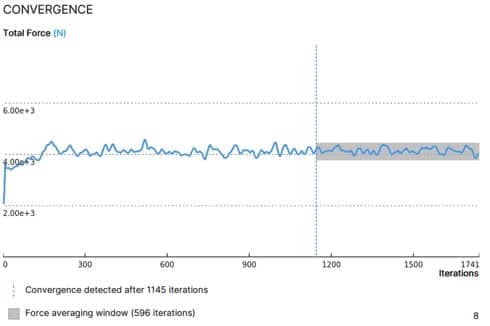
Fig. 6 illustrates the convergence detection and dynamic sizing of the averaging window for a real industrial case. Mind this graph represents the "second" CFD run, on the adaptively refined mesh. It started from the mapped fields from the first, coarse mesh and therefore the initial oscillations are fairly limited. This illustrates the method works well even on a fairly irregular force graph, with a varied "frequency" content.

Interesting links:

Github repository