Concepts for generating lateral aerodynamic forces by means of an asymmetric airflow
Abstract
In this report, the Aquilo AERO concept car of AIRSHAPER has been further investigated, with the objective to improve performance and/or reduce the packaging requirements of the currently patented setup. The open source CFD tool, OpenFOAM, was mainly used during the project. The work was carried out at the CFD department of AIRSHAPER during the third year internship period (7 September 2015 - 29 January 2016) with Mr. Wouter Remmerie as the supervisor.
Summary
This project aims at researching and understanding the aspects of Computational Fluid Dynamics (CFD) through the medium of designing concepts where greater lateral aerodynamic forces can be achieved on a car. CFD software to visualise and analyse the behaviour of a fluid around an object is a necessary tool for making the realisation of such concepts possible. Considering that wind tunnel experiments can be tedious, expensive and inefficient with regards to production time, it is advantageous to execute optimisation processes with CFD. From this project, it is worth to realise that the whole operation of a car, the aerodynamics are the key element for it’s functioning. Aerodynamic forces are points of concern in this project as it is the key driver towards the dynamics of the car and the overall efficiency.
The patented concept within Aquilo AERO aims to counter some portions of the centrifugal forces, which are a product of bend taking by vehicles. This way, the dynamics of a car and its overall efficiency can be improved. For example, higher cornering speeds, a lower fuel consumption and increased safety can be achieved. During the project, a number of concepts have been designed and implemented on a reference car that has been created in CATIA and 3Ds MAX. To investigate these concepts, the CFD tool OpenFOAM is used during the entire project. OpenFOAM is capable of simulating the real life conditions relatively accurately. The K-OmegaSST turbulence model was used, as it accounts for highest accuracy for large flow separations. High computational power was required as it had been decided to use 3000000 cells for all simulations and therefore, the simulations were carried out on a server. By conducting a comparative study of different concepts, the ones with the greatest potential are then implemented on Aquilo AERO, with the intention to achieve greater lateral forces. Theories of fluid dynamics, such as Reynolds Transport Theorem (RTT), Reynolds Averaged Navier-Stokes (RANS), and turbulent flow, were also discussed and studied during the project.
List of symbols
Cd Drag coefficient
Cl Lift coefficient
Cp Pressure coefficient
C𝜇 Turbulent constant model
Fx Force along the a-axis
Fy Force along the y-axis
Fz Force along the z-axis
L Lift force
D Drag force
p Static pressure
p∞ Dynamic pressure
k Turbulent kinetic energy
l Turbulence length
L Characteristic length
V Kinematic viscosity
U Local velocity
U∞ Free stream velocity
epsilon Turbulent dissipation rate
omega Specific dissipation rate
rho Density
A Projected area
Re Reynolds number
List of Terms
| Characteristic length | The length of an object in the flow field. |
| Eddies | Are turbulent patterns also called vortices. |
| Incompressible flow | The density of a fluid element does not change during its motion. |
| Inviscid flow | The flow of an ideal fluid that is assumed to have no viscosity. |
| Kinematic viscosity | The total viscosity of a fluid divided by the fluid mass density. |
| Steady-state | Time-independent. |
| Transient | Time-dependent. |
| Turbulent dissipation rate | Turbulent kinetic energy is converted to thermal internal energy. |
| Turbulence intensity | Turbulence level in [%]. |
| Turbulent kinetic energy | The kinetic energy of the turbulence in a turbulent flow. |
List of abbreviations
| CFD | Computational Fluid Dynamics |
| CV | Control Volume |
| FVM | Finite Volume Method |
| NS | Navier-Stokes |
| OpenFOAM | Open Source Field Operation And Manipulation |
| RANS | Reynolds Averaged Navier-Stokes |
| RE | Reynolds Number |
| RTT | Reynolds Transport Theorem |
| SST | Shear Stress Transport model |
| STL | StereoLithography |
Preface
In this technical report, I will specify my experiences obtained during the third year internship. This report contains an overview of the technical aspects I encountered during the internship timespan. Additionally, the tasks and activities I have worked on at AIRSHAPER, in Antwerpen, Belgium.
Acknowledgement
First and foremost, I want to express my gratitude to my supervisor at AIRSHAPER, M.Eng. Wouter Remmerie, for granting me an opportunity to work on such a challenging and captivating subject. Also, thank you very much for your expert guidance and the continuing patience you had in explaining the steps in using OpenFOAM and the facets of CFD.
I also want to thank my internship supervisor, M.Eng. Arjan Saathoff, for the valuable advices, support and visiting me amid the internship.
Last, but not least, I want to thank my family and my girlfriend Loren for always believing in me and supporting me during the hard times I had during the internship.
Chapter 1
Introduction
Computational Fluid Dynamics (CFD) is a numerical implement that is widely used today for engineering problems. It is the utilisation of applied physics, mathematics and computational program to visualise and analyse how a fluid flows, as well as how a fluid flows past an object. The Automotive & Aerospace industries are examples of fields in which CFD has played a major role in the definition of more aerodynamic shapes.
Background
In 2009, the founder of AIRSHAPER, Wouter Remmerie developed an aerodynamic steering concept for vehicles based on asymmetric airflow [1]. Where conventional race cars apply downforce to increase the traction limit, the concept varies the flow through internal and external air channels to generate lateral forces on the car.
According to the official patent of Aquilo AERO [3], to increase maximal lateral forces one of the techniques is to create downforce, as it applies more pressure on the ground surface. Proportionally, the wheels will encounter a greater contact pressure to the ground surface, by which higher shear forces can be absorbed. A disadvantage of creating downforce is that the load on components such as chassis, suspensions, bearings and tires is higher. These parts need to be given a substantial construction, this having an adverse effect on the total weight of the vehicle. Moreover, higher load results in faster wear of the components, hence, a negative effect in respect of maintenance costs and reliability.
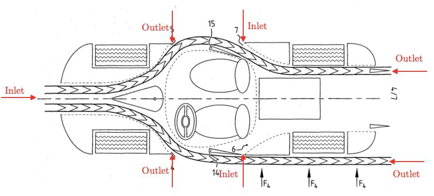
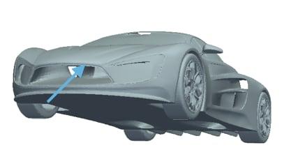
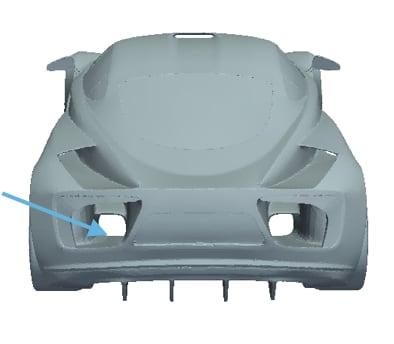
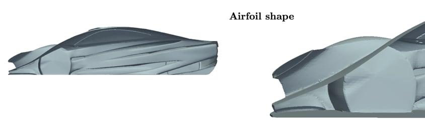
AIRSHAPER has been searching for solutions for absorbing lateral forces when taking bends. As one can see in Fig. (1.1) and Fig. (1.2) channels that extend from an inlet to an outlet are formed in the bodywork, wherein control elements are arranged. The function of a control element is to force an airflow to flow asymmetrically, hence, the lateral force is generated on the car. The intensity of the lateral force can be regulated by to the mobility of the control elements.
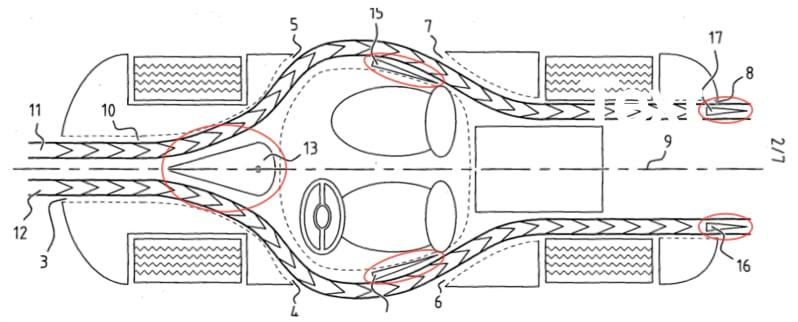
As the concept in its current form has mainly been focused on a rear engined car, much of the unused space in the front of the car was used for internal channels. As one can see in Fig (1.2), the inlet is positioned such that the incoming airflow will flow parallel through the channel, as a consequence of an onward movement of the vehicle. The inlet is branched with two outlet openings on both sides of the bodywork. When a bend is negotiated, the control element will block or partially block one of the branched channels, where the airflow is enforced to flow more in one of two outlets. The air flowing out will further alter the airflow around the vehicle. According to Bernoulli’s principle [5], changing the speed of air results in a change in pressure. Due to the pressure difference on both sides of the vehicle, a lateral force is generated on the side of the car.
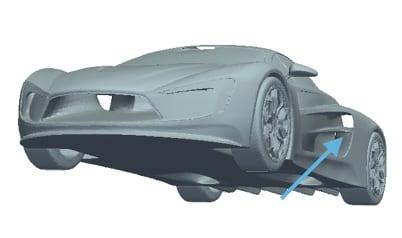
As one can also see in Fig (1.2), two inlets openings are placed on the sides at the rear relative to the two outlets placed at the front. The purpose of this is to let an undisturbed airflow that flows out of the outlet to at least partially flow through the inlet opening. An undisturbed airflow implies that none of the control elements hinder the air from flowing in or out of the channel, the control elements are in neutral position. Such linkage between inlet and outlet openings have been found in tests and CFD simulations to result in better controllability and aerodynamic stability.
The intention of AIRSHAPER with this concept is to create a lateral force that can be employed to counteract a part of the centrifugal forces that result when taking a bend. As a result, an increase in maximum cornering speed can now be achieved without dependency on friction to the ground. Accordingly, by replacing the otherwise necessary downforce, the load on the structural elements are reduced, and this results in lighter components and greater fuel consumption.
Purpose
The main purpose of this internship is to understand computational fluid dynamics. During the project, OpenFOAM is mainly used. OpenFOAM is an open source CFD tool that is well respected in both the academic and industrial world. OpenFOAM appears to be an accurate tool in the automotive industry, for example, Volvo has previously tested cars with OpenFOAM in conjunction with Fluent [2].
To gain knowledge and experience with CFD, the Aquilo AERO project has been improved regarding its aerodynamic performance. The primary task is to generate as much lateral force as possible, through the medium of developing new concepts based on the same principles of the original patent of Aquilo AERO. To perform a comparative study, different concepts were first implemented on a reference car, which was modelled during the project (the basis was a Mercedes S-class coupe). Finally, the concepts that have shown the highest potential were also implemented on the Aquilo AERO concept car and analysed using OpenFOAM.
Approach
Various cases are carried out using the open source CFD tool OpenFOAM. The aim is to design concepts that can generate as much lateral forces as possible, preferably with a small drag and downforce penalty. Due to the lack of previous experience with computational fluid dynamics, it is first necessary to obtain the required knowledge. The following steps have been taken during the internship work:
- Learn the important aspects of CFD. This including the derivation of the Reynolds Transport Theorem (RTT) to the understanding of the continuity, momentum, and the energy equations. For this project, the Finite Volume Method (FVM), or the so-called control volume method will be used.
- Set up cases using different STL files for practice. After that, simulations will be carried out with OpenFOAM. Additionally, for result accuracy a mesh sensitivity analysis will be performed (see Chapter 3).
- A new concept car will be designed in 3Ds MAX and CATIA. Different ideas will be sketched and afterward implemented on the new car.
- Simulations will be performed with a free stream velocity of 55.56 m/s (200 km/h) with no crosswinds. The following hypotheses will be applied for each simulation:
- Reynolds Average Navier-Stokes (RANS)
- Incompressible flow
- Steady-state
- A trade off will be performed to examine the potential of each concept and drag penalty for the generated lateral force.
Boundaries and scope
This project is not intended to cover all aspects of CFD. Fields like unsteady-state (transient) and heat transfer are not included in this project. However, the focal point is aerodynamics. As this is a comparative study of concepts, the total cells used for each simulation is 3000000, considering anything above this number will consume a lot of simulation time. Also, simulations will be depended on previously existing solvers, which implies that it is not required to do programming i.e. amendments to the solvers. Also, due to the limit time, it is not possible to do animations and renderings for the final concept.
Structure
The structure of this report is as follows. Chapter two describes theoretical background that was necessary to acquire prior the start of the project. In chapter three, the simulation setup and mess sensitivity analysis will be described. It is necessary to confirm accurate results before commencing any simulations. Different concepts will be implemented on a generic car in chapter four, which in the same chapter, the aerodynamic results will be discussed and afterward a trade off will be performed. In chapter five, the best concept will be implemented on Aquilo AERO car, which in the same chapter, the aerodynamics results are discussed alongside further ideas to improve the concept car. Chapter six holds the conclusions regarding the improvements on the Aquilo AERO project as well as the recommendations regarding this project.
Chapter 3
Theoretical background
In this chapter, the theoretical background of computational fluid dynamics will be discussed, as well as the software used during the project.
Fluid Dynamics
Reynolds Transport Theorem (RTT)
In this project, the Finite Volume Method (FVM), or the so-called control volume method is used. By definition, a control volume (see Fig 2.1) is an identified region in space across which matter and energy can flow [11].
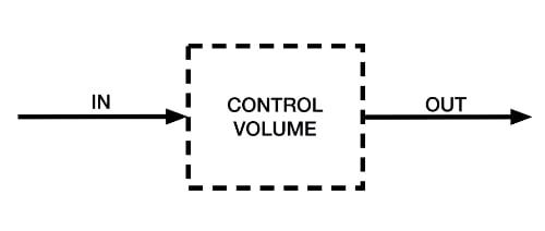
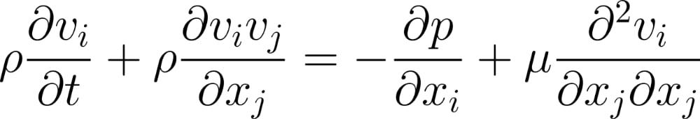
For a CV one can write an equation. However, the complication of writing this equation is in using some of the core laws of mechanics that are not naturally developed for a CV. The Newton’s Laws of motion, those are evolved for identified sets of particles. In other words, the core equations of mechanics are suitable for a Lagrangian description; that is when you have a trajectory of each particle that is ruled by the Newton’s Laws of motion. On the other hand, CV’s are called the Eulerian approach; that is when you are attentive in studying the transport behaviour across that region. For fluid dynamics, it is more suitable to use the Eulerian approach because fluid is constantly reforming. Identifying particles in a fluid can be complicated because many particles will be emerging in very tangled ways unless the flow is very simple. Therefore, by looking at a CV you do not have to track the particles, but you are looking at what is happening in the focused region.
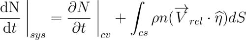
Accordingly, the Eulerian approach is more advantageous. However, the only affair is that the core equations of mechanics are not intrinsically for Eulerian description. To use the Eulerian description and at the same time the fundamental laws of mechanics, we must use the Reynold’s Transport Theorem (RTT). This transformation transforms a Lagrangian description to a Eulerian description. This transformation is described as a mathematical representation in Eq. (2.1). The continuity and momentum equations can be derived from it.
Reynolds Averaged Navier-Stokes (RANS)
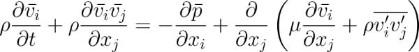
The utilisation of Navier-Stokes equations for simulations exceeds the computational power of most of the supercomputers today. The Reynolds Averaged Navier-Stokes (RANS) equations consist of a modification of the Navier-Stokes equations where the pressure and velocity fields are averaged over time. The NS equation is divided into two components (see Eq 2.2).
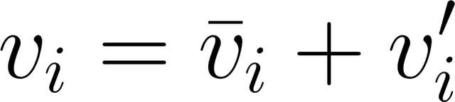
Where Vi_averaged is the time-averaged component and Vi_fluctuation is the turbulent fluctuation term. The fluctuation component depends on the selected turbulent model. As a result, the computer power and simulation times are significantly reduced. The RANS equation is presented as a mathematical form shown equation (2.3).
Turbulent flow
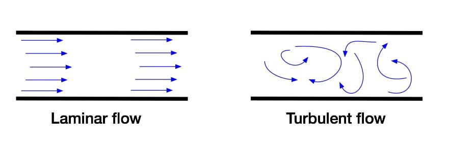
In fluid dynamics there are two main flow regimes, laminar and turbulent flow, see Fig (2.2). In laminar flow, the adjacent layers of fluid have a high degree of orderliness. Thus, the flow is smooth with no eddies or irregular fluctuations. By contrast, turbulent flow is characterised by chaotic fluid motions, and the different fluid layers are mixed. Besides, the velocity and pressure of the fluid fluctuate rapidly over time. Three-dimensionality and diffusivity are also other important factors.
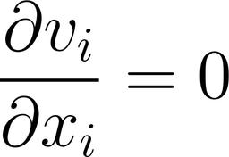
Incompressible turbulent flow is expressed by the continuity equation (2.4) and the Navier-Stokes equation (2.5) as a mathematical representation.
There are many aspects where the type of flow depends on, such as the upstream flow, surface roughness, shape of the object and most importantly the non-dimensional Reynolds Number. The Reynolds number Re is the ratio of the inertial forces to the viscous forces originating in the fluid, see equation (2.6) for its description.
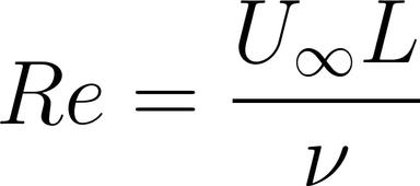
When the critical Reynolds Number Recrit is reached, the transition from laminar flow to turbulent flow take place. Unsteady vortices known as eddies appear in turbulent flow. Large eddies supply continuously smaller eddies with kinetic energy until the energy is dispersed in the smallest eddies, called Kolmogorov scales. Moreover, this evolution is known as the energy cascade. For CFD analyses, it is important to take all the properties of the flow into account, and that is why simulations can be very complex.
Dimensionless quantities
For this project, various aerodynamic coefficients are used, and each of them will be covered in this section.
Drag coefficient
Drag is a crucial aerodynamic force which affects almost everything that moves through air or water. The drag coefficient is critical for aeronautics when designing an aeroplane or automobile as fuel efficiency depends on it. Drag can be described as the resistance force applied to an object moving through a fluid, the faster the object moves through a fluid, the higher the resistance force it will encounter. It is also necessary to bear in mind that drag depends on other factors such as surface roughness, the density of air and laminar or turbulent flow. Drag can be decomposed into two main components:
- Pressure forces: is dependent on the shape of an object (important for bluff bodies)
- Viscous forces: is dependent on skin friction (important for airfoils)

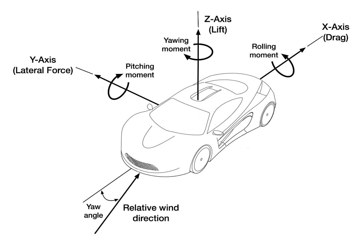
The drag coefficient can be computed using equation (2.7) and is dimensionless. The drag force D shown in the numerator is the force that acts along the x-axis shown in Fig (2.3) and is divided by the dynamic pressure. The A in the denominator is the reference area, since we are looking at a car we take the frontal area into account when calculating the drag coefficient. The frontal area is the projected area along the x-axis shown in Fig (2.3).
Lift coefficient
The lift coefficient is computed likewise. However, the lift force L shown in the numerator of equation (2.8) is the force that acts along the z-axis as shown in Fig (2.3). The reference area A remains the projected frontal area for convenience, when in fact, the projected bottom area would be more related to lift.
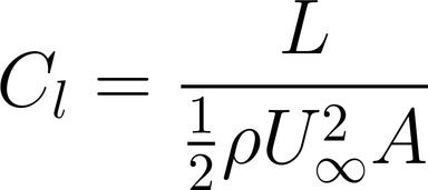
For race cars, generating downforce is preferred as it is advantageous for achieving higher cornering speeds. Downforce is another indication of negative lift force, thus, obtaining negative lift is normal. Whereas, most conventional modern cars have a lift coefficient close to zero or even a positive lift coefficient.
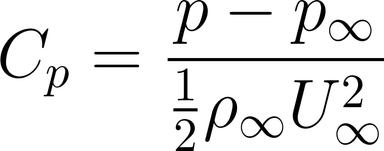
Pressure coefficient
Similarly to the drag and lift coefficient specified earlier, the pressure coefficient is also a dimensionless parameter. The pressure coefficient Cp describes the relative pressure in a fluid flow. The numerator of equation (2.9) states the difference between the local static pressure and the free stream static pressure. This pressure difference is subsequently divided by the free stream dynamic pressure, shown in the denominator.
OpenFOAM
OpenFOAM is short for Open Source Field Operation And Manipulation, which is a free open source CFD software package produced by OpenCFD [3]. It is a well respected CFD tool in both the academic and industrial world. OpenFOAM consists of solvers and utilities. Solvers have the ability to solve problems related to electromagnetics, solid dynamics and complex fluid flows including turbulence and heat transfer. Also, a wide collection of utilities are used for pre and post-processing. As OpenFOAM is programmed to run primarily on Linux, knowledge of this operating system is beneficial.
Solvers
In this section, only the solvers applied to the Aquilo AERO project are described.
simpleFoam
SimpleFoam is a steady-state solver for incompressible turbulent flow. Considering that it is a time-independent (steady-state) solver, and it cannot represent the dynamic formation of eddies, it only gives an averaged solution in the end based on the initial conditions. For time-dependent (transient) simulations there are solvers such as, pimpleFoam and pisoFoam that can present the formation of eddies for each time step.
On a different note, simpleFoam solves a system of RANS equations, which implies that a turbulence model must be specified. During this project, the k-omega SST turbulence model is used for all simulations.
potentialFoam
PotentialFoam is used to initialise the flow field for RANS simulations. Laplace equations are solved to calculate the velocity potential from which the potential field is derived. Since the potential flow is a very basic form a of fluid, turbulence effects cannot be modelled. Therefore, with only using potentialFoam, it is not possible to accurately compute lift and drag.
K-omega SST Turbulence model
For this project, the k-omega SST turbulence model (one of many RANS turbulent models) is used for all simulations. It is based on the k-omega turbulence model, and it also implements k-epsilon, which is widely used nowadays for engineering applications. For this model, the eddy viscosity formulation is modified to account or the transport effects of turbulent shear stress. Also, for large flow separations, the SST model accounts for highest accuracy [6].
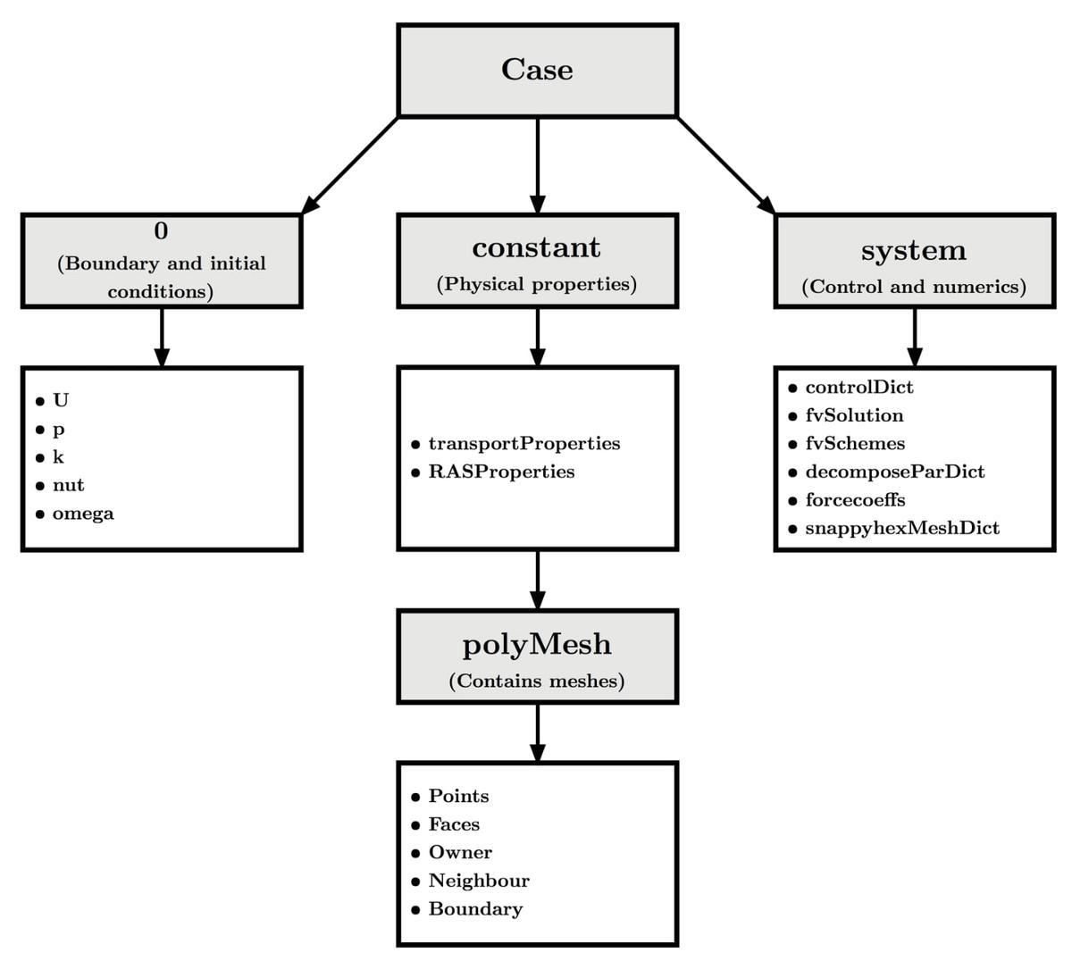
File structure
As OpenFOAM has no GUI (Graphical User Interface), one has to be familiar with the command-line interface. Figure (2.4) intends to explain the general structure for RANS cases.
In the main directory, there are three folders, system, constant and 0. The system directory contains control settings, and these can be changed by altering the controlDict file. In the controlDict file, it is possible to modify the start and end time, write intervals, and solvers. By adding the forceCoeffs file to the controlDict file as a function, one can calculate the aerodynamic coefficients for 3D and 2D object. The fvSchemes file contains discretisation schemes. Also, the fvSolution file contains setting for different solvers.
To change the turbulence and material properties, one have to go to the constant directory. The RASProperties file includes choices between laminar or turbulent flow and a RANS turbulence model. In the transportProperties file, one can define the kinematic viscosity (nu). Also, the polyMesh folder contains all the meshes of the geometry.
Finally, the 0 folder contains all the initial and boundary conditions. For the initial conditions, U is the velocity, p is the pressure, k is the turbulent kinetic energy, nut is the turbulent viscosity (not needed for k-omega SST) and finally omega is the specific turbulence dissipation rate. For boundary conditions, the patches of the box (wind tunnel) around the object must be defined. For example, the front patch should be specified as velocity inlet and rear patch as velocity outlet, only if the velocity is known/defined. Each boundary condition has other options, for example, one can specify the direction of the velocity along (x,y,z).
The content of all the case files for this project can be found in Appendix A.
Chapter 3
In this chapter, the simulation setup for all cases will be described, alongside the mesh sensitivity analysis.
Simulation setup
The simulation setup for all cases are identical and hence this chapter for describing the procedure. At the start of the project, the primary task was to try to find the best simulation settings. OpenFOAM offers many great tutorials, the motorBike tutorial suited best since we are dealing with a vehicle and was used as a base for the simulations setup. Initially, the function of each command inside the different files (see Appendix A) were studied. Afterwards, several random STL files were used to test different setting and also to get hands on OpenFOAM.
To carry out a simulation one must first input meshes into OpenFOAM and this can be achieved in several different ways. At AIRSHAPER, the snappyHexMesh meshing tool is used that comes with OpenFOAM. By configuring the dictionary file snappyHexMeshDict (see Appendix A.1) to get nice meshes can be a very strenuous task. It is a combination of proper geometry and settings that result in a good mesh. To check the quality of the mesh, the checkMesh utility is used.
Once the mesh quality is good enough, the initial conditions and boundary conditions are set. For all simulations, a velocity of 55.56 m/s (200 km/h) is set along the positive x-axis only, which implies no crosswinds. The frontal area of the car is 2.14 m2 and length is 5.027 m. The turbulent settings are shown in (Table 3.1)
Afterwards, the files under the system folder have to be set. In controlDict, the start time is set to 0 and end time to 1000 to give sufficient time for the airflow to stabilise around the car and the wake to obtain accurate results. Also, the forcecoeffs is set as a function in controlDict, to get forces, moments and aerodynamic coefficients.
| Velocity [m/s] | 55,56 |
| Length of car[m] | 5,027 |
| RE[-] | 18618518 |
| Kinematic viscosity [m2/s] | 0,000015 |
| Turbulence Intensity [%] | 8 |
| Turbulence Model constant C𝜇 [-] | 0,09 |
| Turbulent length scale [-] | 0,35189 |
| TurbulentKE [-] | 29,63 |
| Epsilon [-] | 75,31 |
| TurbulentOmega [-] | 0,39 |
Table 3.1: Turbulent settings
Therefore, a lot of computational power is needed and the simulations were done on a server. A 8 core Intel Xeon E5 was used with 16 Gb of RAM. The simulation processes are divided over each core by using the decomposeParDict under the system folder.
After the simulations are finished, the reconstructPar command combines the results that were divided over the cores. Afterwards, the results were visualised using the post-processing tool paraFoam that comes with OpenFOAM.
Chapter 4
Concepts applied to a generic car
This chapter aims to describe each concept and the results obtained from simulations.
Concept descriptions
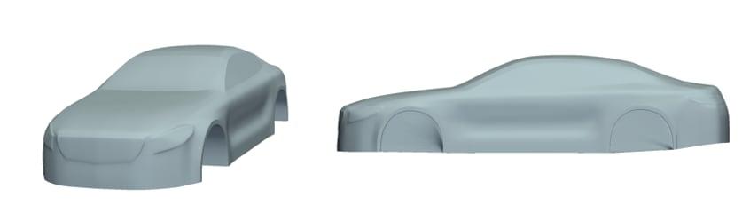
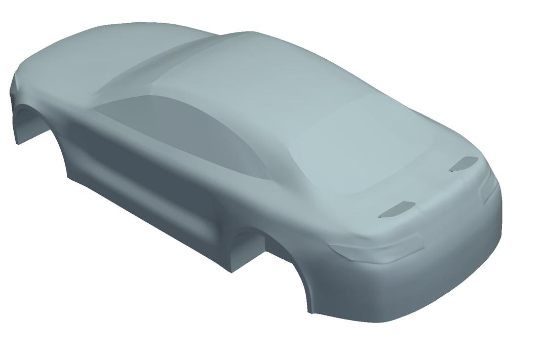
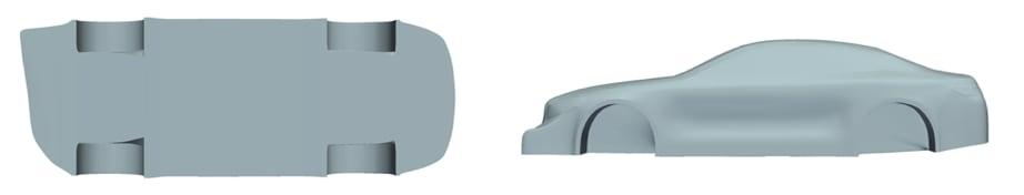
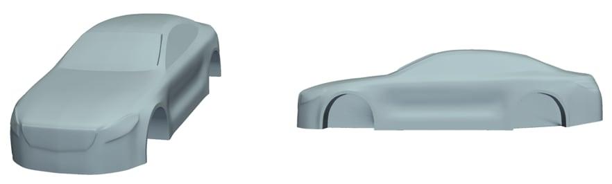
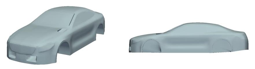
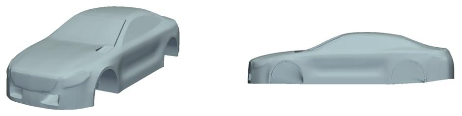
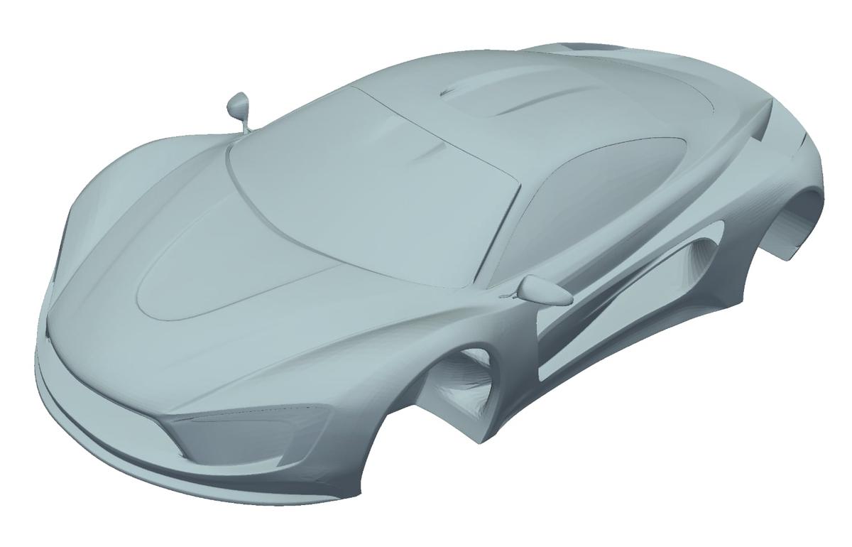
Before coming up with concepts, a reference car has been built in CATIA at first (see Fig. 4.1). The Mercedes S-class coupe 2015 is used as a base of this car. The real dimensions of the vehicle have been taken into account. Due to difficulties working with 3D models in CATIA the car was subsequently made in 3Ds MAX. Without the use of the 3DConnexion Space Mouse it would have been impossible to work in 3D. A simulation was performed on this reference car to obtain forces and moments that will serve as a basis for comparison with the other concepts.
Concept 1
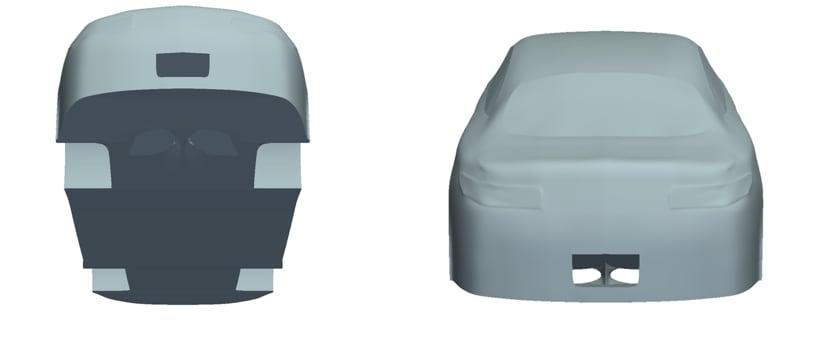
In this concepts, to inlets at the front, just below the radiator, lead the air through internal channels to outlets just below the front windshield as seen in (Fig 4.2). At high speed, if the vehicle takes a bend to the right, the right channel will close and vice-versa. The open channel will cause the airflow to “collide” with the standard airflow that goes around the A-pillar, creating a low pressure zone on that side of the vehicle. The aim is to create a high-pressure zone and a low-pressure zone on either side of the vehicle depending on the bend. Due to the pressure difference, lateral force can be generated on the vehicle.
Concept 2
For this concept, two flaps are placed at the rear as seen in (Fig. 4.3). If both are extended downforce can be created. However, the aim with this concept is to extend or retract one flap at a time causing downforce at only one side of the vehicle.
Concept 3
For this concept, the front bumper can partially extend and retract as seen in (Fig. 4.4). The aim of this concept is to direct the main flow to either the left or right side of the vehicle, thus creating an asymmetric flow pattern and with it a lateral force. However, the first goal is to assess the potential of this concept before thinking of practical implementations (which do not appear to be straightforward for this concept). Afterwards, if succeeded the mechanics can be considered
Concept 4
For this concept, a gurney flap is placed on the A-pillar as seen in (Fig. 4.5). The gurney flap can rotate depending on which side the turn is taken. Like all the other concepts, the aim is to disturb to flow on either side of the vehicle causing the airflow to flow rapidly over the A-pillar. Hence, a low-pressure zone and a high-pressure zone can be achieved which results in lateral forces.
Concept 5
This idea came from the Aquilo AERO concept car, as it has two inlet channel at the bottom and two outlets at the rear. For this concept, the two outlets are combined to see how it effects the vehicle, see (Fig. 4.6). If both channels are open downforce can be generated on both sides, otherwise, on only one side of the vehicle.
Aerodynamic results
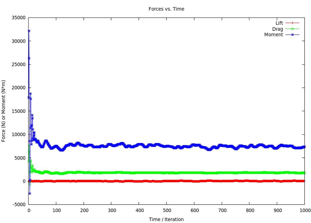
The first results for the reference car appeared to have slight lateral force and downforce already. For a car that is symmetrical, it is expected that lateral force should be around 0 [N]. A first explanation could be model inaccuracies. But although the model was relatively basic, it was perfectly symmetric, as was the mesh itself. A second explanation was that the forces and moments were extracted at one point in time, where they could be at a peak value due to oscillations. Averaging was therefore applied to cancel out this effect and see whether it explained the lateral forces or not.
By plotting the lift, drag and moment against the number of iterations, it can be seen where the forces stabilise, see (Fig. 4.7). It is sometimes necessary to zoom in the plots to see approximately where the patterns repeat between an interval, see (Fig. 4.8). By looking at the red line (lift) for example, it can be seen that from 350 to 450 iterations the pattern repeats. Therefore, by averaging the forces and coefficients between this interval will give you accurate results.
![Figure 4.8: Force vs. time plot [300-600 iterations]](/_next/image?url=%2Fassets%2Fresearch%2Fimages%2Fsports-car-aerodynamics%2Ffigure48.jpg&w=1080&q=75)
The difference in results can be seen in the following table:
| Concepts | Forces [N] | ||
|---|---|---|---|
| Fx | Fy | Fz | |
| Reference Car | 1320 | 54 | 155 |
| Reference Car Averaged | 1446 | 3 | 28 |
Table 4.1: Comparison between results
It can be seen that the lateral force is close to 0, and lift decreased drastically. This method is thus applied for all other concepts to obtain accurate results.
Concept 1
For this concept, one channel was blocked to see if lateral force are generated. From the results obtained, it can be concluded that there is no lateral force created at all. Drag and downforce are increased only. See (Table 4.2) for the result compared to the reference car.
| Concepts | Force Coefficients | Forces [N] | Length [m] | Frontal Area [m2] | |||
|---|---|---|---|---|---|---|---|
| Cd | Cl | Fx | Fy | Fz | |||
| Reference Car | 0,35 | -0,036 | 1446 | 3 | 28 | 5,027 | 2,14 |
| Concept 1 | 0,37 | -0,0337 | 1527 | 2 | -323 | 5,027 | 2,14 |
Table 4.2: Comparison between concept 1 and reference car
Concept 2
For this concept, one flap was in the retracted positions and the other one extended. From the results obtained, it can be concluded that some lateral force is being generated, and a lot of downforce. See (Table 4.3) for the result compared to the reference car.
| Concepts | Force Coefficients | Forces [N] | Length [m] | Frontal Area [m2] | |||
|---|---|---|---|---|---|---|---|
| Cd | Cl | Fx | Fy | Fz | |||
| Reference Car | 0,35 | -0,036 | 1446 | 3 | 28 | 5,027 | 2,14 |
| Concept 2 | 0,35 | -0,0150 | 1423 | 56 | -468 | 5,027 | 2,14 |
Table 4.3: Comparison between concept 2 and reference car
Concept 3
For this concept, one side of the front bumper was extended. From the results obtained, it can be concluded that significant amount of lateral force is being generated, and some downforce. See (Table 4.4) for the result compared to the reference car.
| Concepts | Force Coefficients | Forces [N] | Length [m] | Frontal Area [m2] | |||
|---|---|---|---|---|---|---|---|
| Cd | Cl | Fx | Fy | Fz | |||
| Reference Car | 0,35 | -0,036 | 1446 | 3 | 28 | 5,027 | 2,14 |
| Concept 3 | 0,36 | -0,015 | 1429 | -118 | -69 | 5,027 | 2,14 |
Table 4.4: Comparison between concept 3 and reference car
Concept 4
For this concept, the gurney flap was in extended position only at one side of the A-pillar. From the results obtained, it can be concluded that great amount of lateral force is being generated, and a lot of lift See (Table 4.5) for the result compared to the reference car.
| Concepts | Force Coefficients | Forces [N] | Length [m] | Frontal Area [m2] | |||
|---|---|---|---|---|---|---|---|
| Cd | Cl | Fx | Fy | Fz | |||
| Reference Car | 0,35 | -0,036 | 1446 | 3 | 28 | 5,027 | 2,14 |
| Concept 4 | 0,37 | -0,0936 | 1513 | -191 | 342 | 5,027 | 2,14 |
Table 4.5: Comparison between concept 4 and reference car
Concept 5
For this concept, one channel was blocked. From the results obtained, it can be concluded that small amount of lateral force is being generated, and a lot of downforce See (Table 4.6) for the result compared to the reference car.
| Concepts | Force Coefficients | Forces [N] | Length [m] | Frontal Area [m2] | |||
|---|---|---|---|---|---|---|---|
| Cd | Cl | Fx | Fy | Fz | |||
| Reference Car | 0,35 | -0,036 | 1446 | 3 | 28 | 5,027 | 2,14 |
| Concept 5 | 0,36 | -0,0482 | 1469 | -22 | -181 | 5,027 | 2,14 |
Table 4.6: Comparison between concept 5 and reference car
Trade-off
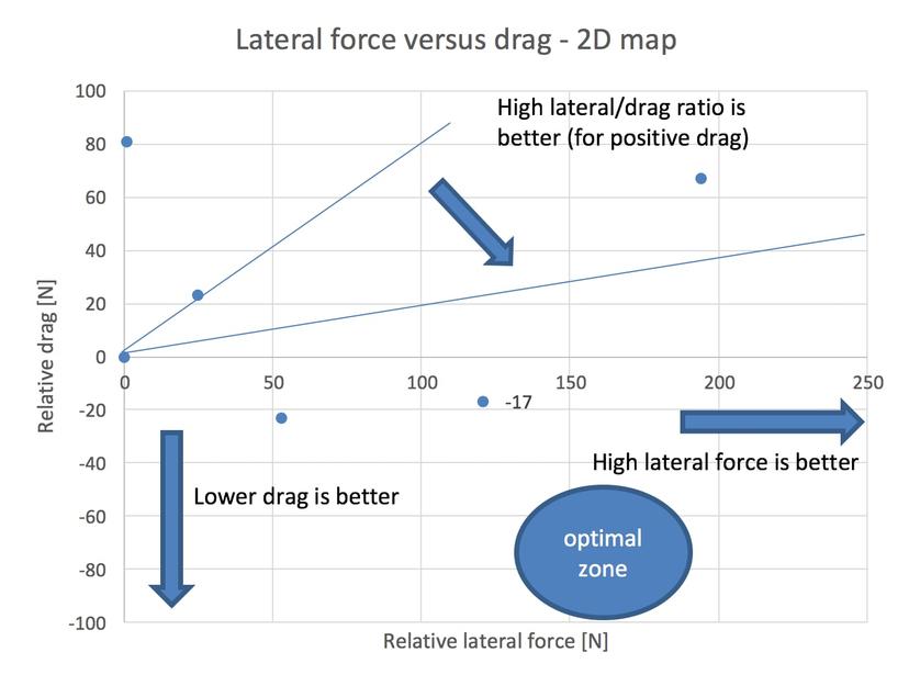
By choosing the best concept(s) a trade-off must be performed. By plotting the results, with the lateral force on the x-axis and drag on the y-axis shown in (Fig. 4.9), some concepts can be eliminated. It should be noted that relative forces are used here. Additionally, these are the three important criteria for this project:
- Generates high amount of lateral force.
- No drastic increase in drag.
- Easy to implement on a race car.
| Concepts | Force Coefficients | Forces [N] | Length [m] | Frontal Area [m2] | |||
|---|---|---|---|---|---|---|---|
| Cd | Cl | Fx | Fy | Fz | |||
| Reference Car | 0,35 | -0,036 | 1446 | 3 | 28 | 5,027 | 2,14 |
| Concept 1 | 0,37 | -0,0337 | 1527 | 2 | -323 | 5,027 | 2,14 |
| Concept 2 | 0,35 | -0,1150 | 1423 | 56 | -468 | 5,027 | 2,14 |
| Concept 3 | 0,36 | -0,015 | 1429 | -118 | -69 | 5,027 | 2,14 |
| Concept 4 | 0,37 | -0,0936 | 1513 | -191 | 342 | 5,027 | 2,14 |
| Concept 5 | 0,36 | -0,0482 | 1469 | -22 | -181 | 5,027 | 2,14 |
Table 4.7: All concepts vs. reference car
From (Fig. 4.9), the following conclusion can be given for each concept.
Concept 1: This concept does not generate lateral force at all. It creates also more drag. Therefore, this concept drops out.
Concept 2: This concept does generate some lateral force. It has also a small penalty for drag and creates a lot of downforce. This concept has been seen on Pagani cars. It is an interesting concept but cannot be used.
Concept 3: This concept generates quite some lateral force, and it is good for drag and downforce. However, it is mechanically complex. Also, impossible to implement on Aquilo Aero as it has a small front bumper.
Concept 4: This concept generates a high amount of lateral force but needs improvements on the drag penalty. This concept is very interesting as it is mechanically simple. It is clear that this concept scores the best, and therefore, it will be investigated and implemented on the Aquilo AERO concept car.
Concept 5: This concept generates not enough lateral force. Although, it functions well as a diffusor to generate downforce.
Chapter 5
Concepts applied to Aquilo AERO
This chapter aims to describe the concepts that are applied to the Aquilo AERO car and the results obtained from simulations.
Combining concepts
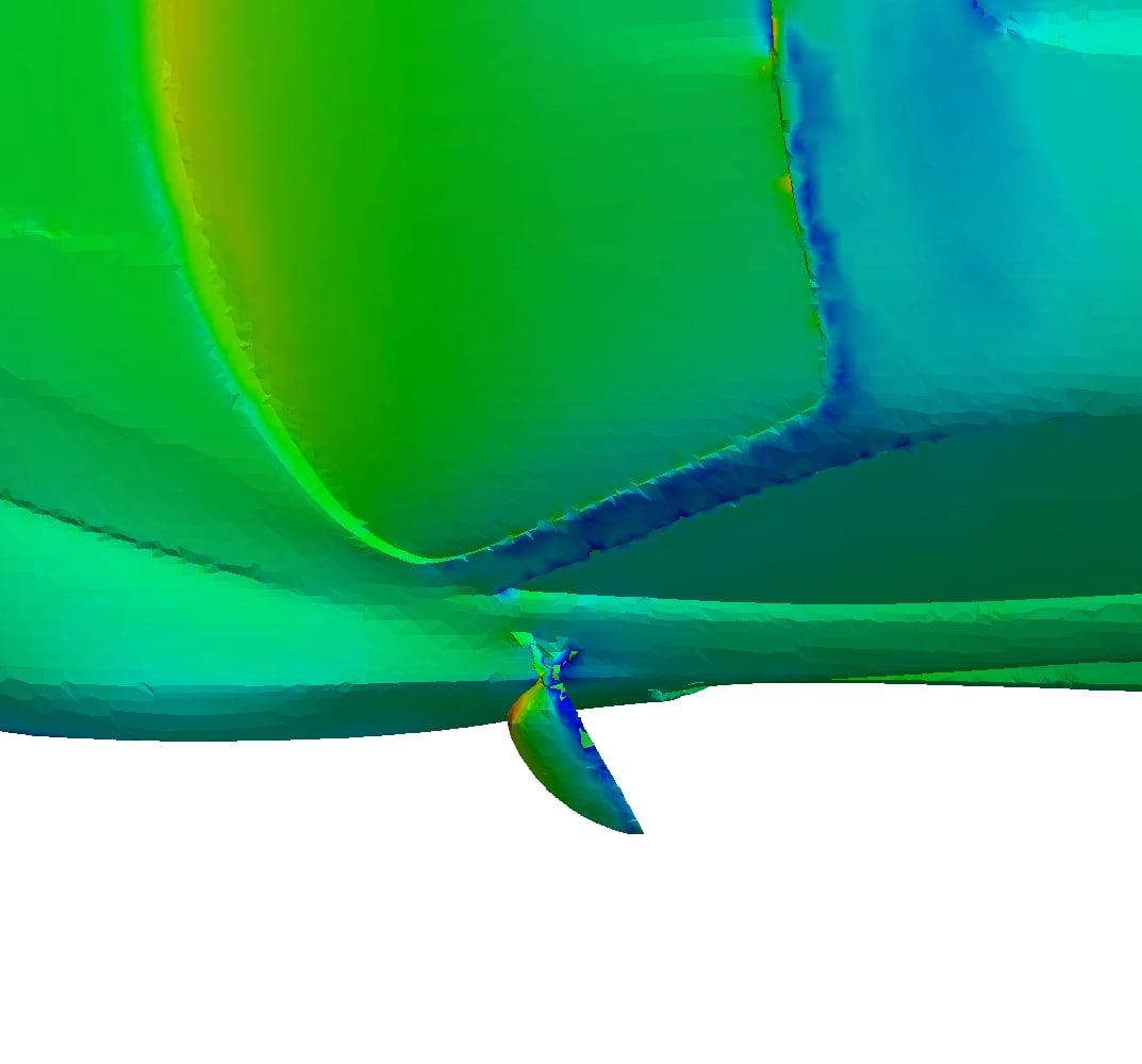
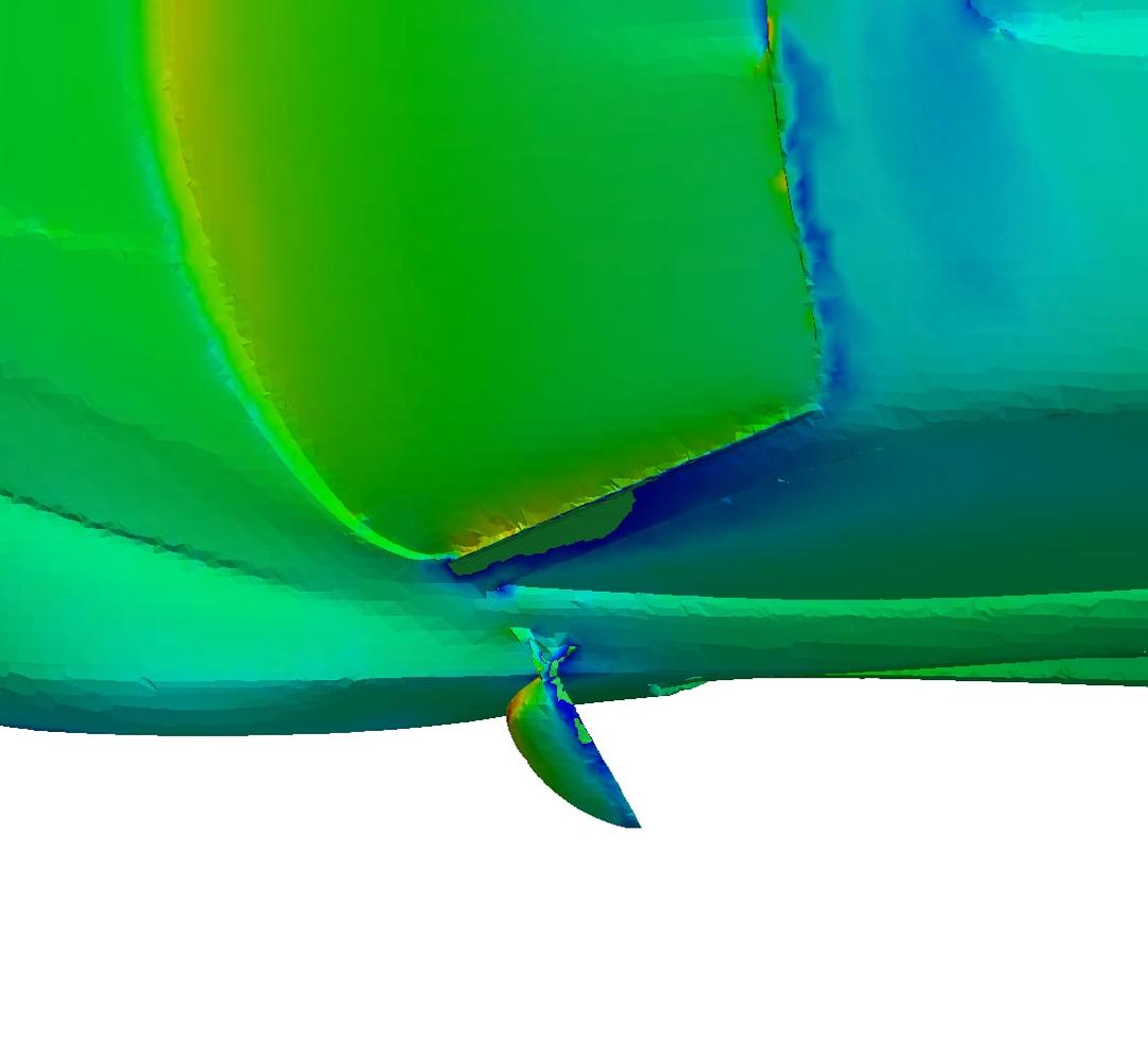
Before implementing concept 4 on Aquilo AERO, it has been decided to combine concept 1 with 4. The purpose of this is to see wether the air channels in concept 1 increases the airflow around the A-pillar. Thus, it is possible to disturb the airflow more when the gurney rotates or extends when a turn is negotiated. There are two versions simulated, one with a normal gurney and the other with an extended (longer) gurney, see (Fig. 5.1 and 5.2).
Aerodynamic results
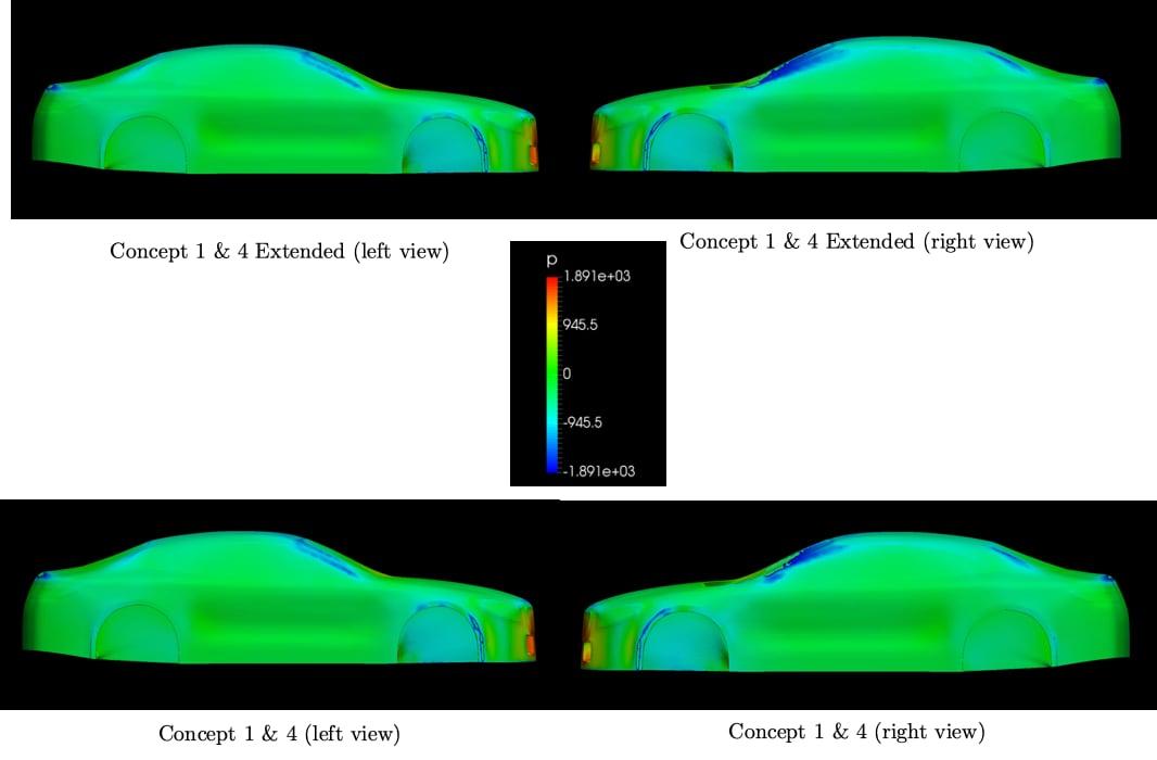
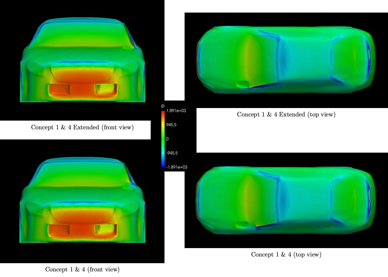
As it can be seen in (Table 5.1), concept 1 & 4 generates less lateral force than the standalone concept 4 as shown in (Table 4.7), the difference is ≈20 [N]. For concept 1 & 4 with the extended gurney flap, higher lateral forces are obtained, the difference is ≈50 [N]. Please note, the simulation results shown in the table below are averaged as discussed in (Chapter 4.2). Additionally, see (Appendix B.1) for the pressure distribution for both concepts.
| Concepts | Force Coefficients | Forces [N] | Length [m] | Frontal Area [m2] | |||
|---|---|---|---|---|---|---|---|
| Cd | Cl | Fx | Fy | Fz | |||
| Reference Car | 0,35 | -0,036 | 1446 | 3 | 28 | 5,027 | 2,14 |
| Concept 1 + 4 | 0,38 | -0,0813 | 1545 | -172 | -417 | 5,027 | 2,14 |
| Concept 1 + 4 extended gurney flap | 0,39 | -0,1106 | 1562 | -240 | -466 | 5,027 | 2,14 |
Table 5.1: Comparison between combined concepts and reference car
In order to improve Aquilo AERO, it is important to carry out the same steps executed for the generic car done in (chapter 4). First, the Aquilo AERO reference car is simulated with a clean setup (open channels), this is important as everything else will be compared to this result. Afterwards, each channel is blocked separately and subsequently simulated. This is to quantify the performance of the existing, patented concept. This will serve as a bench mark for the new concepts. Finally, the Aquilo AERO car is set up with an asymmetric setup and later on the gurney flap was implemented on the A-pillar with the same setup.
To have a better understanding which channels have been blocked, see the figures below. Please note, for an asymmetric setup all three channels are blocked.
| Concepts | Force Coefficients | Forces [N] | Length [m] | Frontal Area [m2] | |||
|---|---|---|---|---|---|---|---|
| Cd | Cl | Fx | Fy | Fz | |||
| Aquilo Reference | 0,39 | -0,6836 | 1241 | -28 | -2190 | 4,4 | 1,715 |
| Aquilo 1 | 0,38 | -0,6753 | 1232 | -58 | -2185 | 4,4 | 1,715 |
| Aquilo 2 | 0,38 | -0,3542 | 1217 | -218 | -1151 | 4,4 | 1,715 |
| Aquilo 3 | 0,39 | -0,6275 | 1244 | -165 | -2030 | 4,4 | 1,715 |
| Aquilo Asymmetric | 0,38 | -0,3510 | 1218 | -270 | -1118 | 4,4 | 1,715 |
Table 5.2: Comparison between Aquilo reference car and different setups
From the results shown in (Table 5.2), it can be seen that for the asymmetric setup, 270 [N] is generated. The Aquilo AERO car was calculated in the past with a free stream velocity of 83.33 m/s (300 km/h), and it generated 300 [N] of lateral force. The main difference is due to the much coarser mesh on the original study. The present results are much more accurate. It can also be seen that channel 2 (Aquilo 2) generates the highest amount.
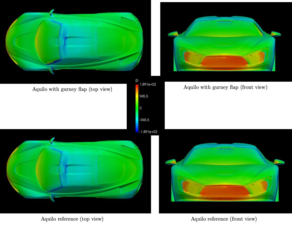
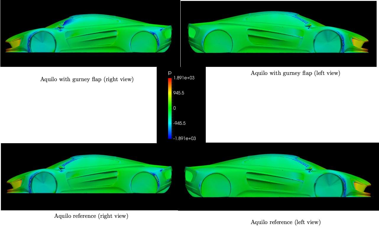
Finally, the gurney has been implemented on the A-pillar of the Aquilo AERO concept car, see (Fig. 5.6). Afterwards, simulations have been carried out, see (Table 5.3) for the results.
| Concepts | Force Coefficients | Forces [N] | Length [m] | Frontal Area [m2] | |||
|---|---|---|---|---|---|---|---|
| Cd | Cl | Fx | Fy | Fz | |||
| Aquilo Reference | 0,39 | -0,6836 | 1241 | -28 | -2190 | 4,4 | 1,715 |
| Aquilo + Gurney | 0,40 | -0,7067 | 1280 | -118 | -2237 | 4,4 | 1,715 |
Table 5.3: Comparison between Aquilo reference car and Aquilo + gurney flap
It can be seen that with the gurney flap, it has now an additional 90 [N] of lateral force. This is a lot less compared with the gurney flap situated on the generic car. In (Table 4.5), it can be seen that the gurney flap generates ≈190 [N] on the reference car. a possible explanation could be the more inclined A-pillar of the Aquilo car (lower angle with respect to the ground, so a flatter A-pillar). This could make it easier for the air to get around the A-pillar and the gurney and thus a reduced effect on the lateral pressure on the car. Also, the Aquilo AERO car with the gurney has been simulated with blocked channels (asymmetric), see (Table 5.4).
| Concepts | Force Coefficients | Forces [N] | Length [m] | Frontal Area [m2] | |||
|---|---|---|---|---|---|---|---|
| Cd | Cl | Fx | Fy | Fz | |||
| Aquilo Reference | 0,39 | -0,6836 | 1241 | -28 | -2190 | 4,4 | 1,715 |
| Aquilo Asymmetric + Gurney | 0,38 | -0,3619 | 1264 | -356 | -1151 | 4,4 | 1,715 |
Table 5.4: Comparison between Aquilo reference car and Aquilo Asymmetric+ gurney flap
Further improvements
To improve Aquilo AERO to another level, a new concept has been considered. The idea is to increase the airflow around the A-pillar as the internal air channels cannot do that as they exits the flow below the side mirrors. The purpose of this idea is to disturb the airflow more with the gurney as the airflow goes around the A-pillar faster. Hence, a bigger pressure difference can be generated which results in greater lateral forces.
As seen on (Fig. 5.7), the internal front channels are removed. The front windshield of the car is tangent to the hood to let the airflow stream nicely over the car. Afterwards, two splitters are implemented at the front to control the direction of the airflow to flow towards the A-pillar, see (Fig. 5.8). The shape of the splitters is rather simple, it is wether to see if this concept has potential or not. Unfortunately, due to approaching the end of the internship timespan, it was not possible to do simulations for this concept.
Chapter 6
Conclusion and recommendations
This project aims at new concepts where greater lateral aerodynamic forces can be generated. The key task for the internship was to obtain knowledge and experience with Computational Fluid Dynamics (CFD), through the medium of developing new concepts for Aquilo AERO.
A new reference car was built in CATIA and subsequently 3Ds MAX. The results for the reference car were used a base for comparing it with other concepts. During the internship timespan, five concepts were first sketched and implement on the reference car. After performing a trade-off, the gurney concept showed the highest potential with respect to both lateral force and practical implementability.
Also, after the trade-off had been conducted, the concepts with highest potential were combined with concept 1. The gurney flap was also extended more to the hood to see if more lateral force can be generated. Even though concept 3 also has great potential, it was left out. This was due to the difficult implementation on the Aquilo AERO’s front bumper. With the gurney flap implemented on the Aquilo AERO car, it has now an additional ≈100 [N] of lateral force. However, these results are obtained from steady-state simulations. It is recommended to perform crosswind, rotating wheels and transient simulations as it has a significant effect on the results. On a different note, the finer the mesh, the more computational power is required and therefore, it would be worth to try to simulate with perhaps 10 million cells instead of 3 million cells.
Finally, the front air channels of Aquilo AERO have been removed as they do not increase the airflow around the A-pillar. A new concept has been implemented to make this possible. However, simulations were not carried out, due to the fact the internship period concluded.
Recommendations for further work:
- Try out a transient (unsteady case) simulation for Aquilo AERO, including rotating wheels.
- Investigate the cause of the high drag for Aquilo AERO, even though the car looks aerodynamically smooth and stable. Excluding the wheels had some influence on drag, however, not to a vast extent.
- Try out slant angle (crosswind) simulations for Aquilo AERO.
- The standard meshing tool snappyHexMesh provided by OpenFOAM is a bit indefinite and difficult to choose the right settings. Another drawback is that it is not automated. Therefore, everything should be done manually, which can consume a lot of time. Try out different meshing tools, like PointWise and GMSH where it is also exportable to OpenFOAM.
- For result verification and accuracy, it is best to use another CFD package for comparisons like Solidworks and Fluent.
- Discuss the concepts with manufacturers.
- Further improve the gurney concept, as it is an easy add-on that has little impact on the car.
Bibliography
[1] Remmerie, W. (2015). AIRSHAPER. Retrieved from https://airshaper.com
[2] Nebenführ, B. (2010). OpenFOAM: A tool for predicting automotive relevant flow fields. Retrieved from http://www.tfd.chalmers.se/~lada/postscript_files/Bastian-Nebenfuhr-OpenFOAM_A_tool_for_predicting_automotive_flow_fields.pdf
[3] Remmerie, W. (n.d.). Aquilo AERO official patent. Retrieved from http://worldwide.espacenet.com/publicationDetails/originalDocument?CC=WO&NR=2013049900A1&KC=A1&FT=D&ND=4&date=20130411&DB=worldwide.espacenet.com&locale=en_EP
[4] OpenFOAM official website. (n.d.). Retrieved from http://www.openfoam.com
[5] Bernoulli’s principle. Retrieved from - https://www.grc.nasa.gov/www/k-12/airplane/bern.html
[6] SST k-omega model. Retrieved from - http://www.cfd-online.com/Wiki/SST_k-omega_model
[7] Versteeg, H. K., & Malalasekera, W. (2007). An Introduction to Computational Fluid Dynamics (2nd ed.). Essex CM20 2JE, England: Pearson Education.
[8] Anderson, John David. Fundamentals of aerodynamics / John D. Anderson, Jr. — 5th ed. p. cm. — (McGraw-Hill series in aeronautical and aerospace engineering)
[9] Turbulence dissipation rate. (n.d.). Retrieved from http://www.cfd-online.com/Wiki/Turbulence_dissipation_rate
[10] Turbulence kinetic energy. (n.d.). Retrieved from http://www.cfd-online.com/Wiki/Turbulence_kinetic_energy
[11] Computational Fluid Dynamics - Online course. (n.d.). Retrieved from http://nptel.ac.in/courses/112105045/
Appendix B
Pressure maps (Reference car)
Pressure maps (Aquilo AERO)
Download Original Paper