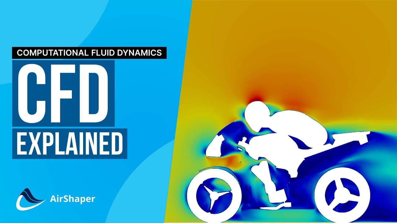
What is Computational Fluid Dynamics (CFD)?
Most of the world around us is affected by fluid dynamics in some way. The aerodynamics of the cars we drive, the hydrodynamics of a tidal power turbine, the aeroacoustics of wind turbines - even the way the wind blows around our cities. In an ideal world, the forces and flows in all these examples would be measurable in an accurate and repeatable way. However, this is often not possible, so engineers have to simulate these flows instead using Computational Fluid Dynamics (CFD).
CFD uses numerical analysis to model the flows and pressures around objects. It runs simulations on Computer Aided Design (CAD) models of the object of interest and calculates the drag and lift forces as well as the surrounding flow field. This allows engineers to study complex flow behaviours and investigate the effects of design changes.
CFD analysis can also simulate curved flow cases and internal flows that cannot be achieved in wind tunnels, helping engineers understand fluid motion in refrigerators and jet engines. These benefits make CFD a powerful tool, that is in demand across many industries.
There are three main stages involved in modelling the flow around an object: modelling, discretisation and linearisation.
CFD modelling
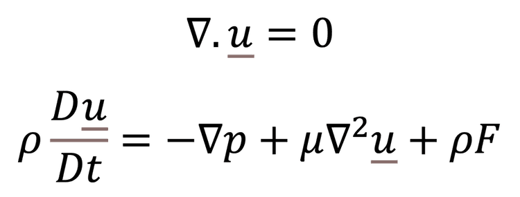
At the heart of the mathematical models used in CFD are the Navier Stokes equations. These are a set of Partial Differential Equations (PDE) which give flow velocity in three dimensions and can be used to calculate other parameters such as pressure and temperature.
The first equation simply represents the conservation of mass in all three dimensions. The second equation is a fluid dynamic form of Newton’s second law (F=ma). Between them, they describe the fundamentals of the flow field. The fluid can’t appear or disappear (conservation of mass) and the acceleration of a mass or volume of fluid is caused by forces due to pressure, viscosity and external forces such as gravity or electromagnetism.
Depending on the application, other equations may be required such as thermodynamic equations, if there are significant temperature gradients or heat sources to consider. Although it is possible to solve the above equations for simple problems, such as laminar flow in a pipe, for anything more complex, it isn’t as straightforward.
Analytical solutions (ones that can be calculated directly over an infinite number of points) don’t exist for most things of interest. In fact, solving the Navier Stokes equations is such a problem, that it forms one of the million-dollar Millennium Prizes for mathematicians.
This would seem to limit the use of the equations, but this is where engineers and mathematicians take divergent paths. The latter are interested in fully understanding the equations and why they don’t always solve. The former are interested in their application to real world problems and have computational tools to approximate solutions to partial differential equations. If done well, the equations work perfectly for most applications.
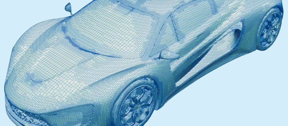
Discretisation or meshing
Discretisation is the process of breaking down an object into discrete points or nodes. This approach is used in Finite Element Analysis (FEA) and in CFD, it is known as meshing. It essentially divides a highly non-linear problem into a very large number of smaller, simpler sections which are considered to be linear. The combination of individual solutions for the points makes up an approximation of the overall solution. Computers are very good at solving large numbers of linear problems so we can approximate our non-linear system relatively quickly.
Another way to think about meshing is to consider digital photographs. Compared to analogue photographs, digital photographs are made up of small blocks, or pixels. The higher the number of pixels, the higher the resolution and the more detail the image will capture. Similarly, to achieve an accurate numerical solution in CFD, ideally you want a high number of nodes in a mesh. However, this requires a lot of computing time to solve all the points, which can be expensive. Instead, there is a balancing act between accuracy and time.
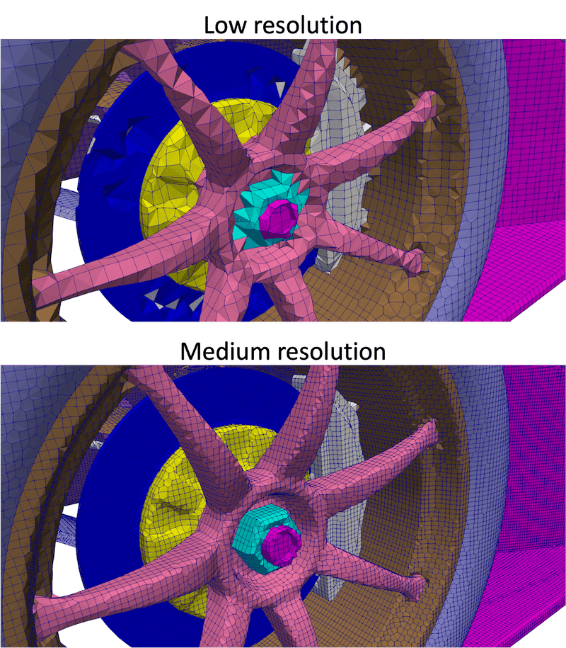
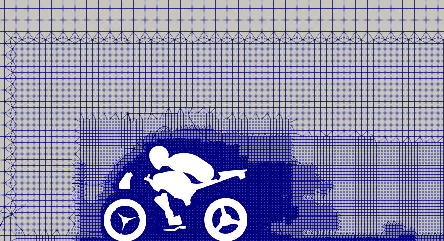
To help reduce computational time, the resolution of the mesh can be modified. For example, a higher resolution mesh is usually required near the surface of the object to capture the behaviour of the boundary layer. While a lower resolution can be used far away from the object. This is how AirShaper's adaptive mesh refinement works.
Iterating the solution
Once the model has been formulated and the mesh created, the equations are solved by a process of iteration. Gaussian elimination or Lower-Upper (LU) decomposition can give a very accurate solution, but given the other sources of error, are usually not worth the extra computational time.
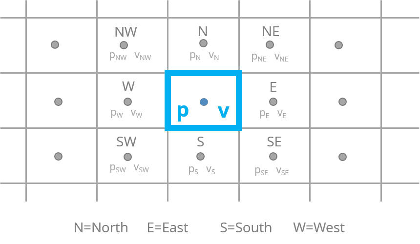
In iterative solutions, the user will set an array of starting conditions and complex solver algorithms will work on each point on the mesh. Each node is subject to the forces due to the surrounding nodes (usually differences in pressure or viscosity due to velocity differences). Each of those surrounding nodes has forces due to other nodes acting on it and so on.
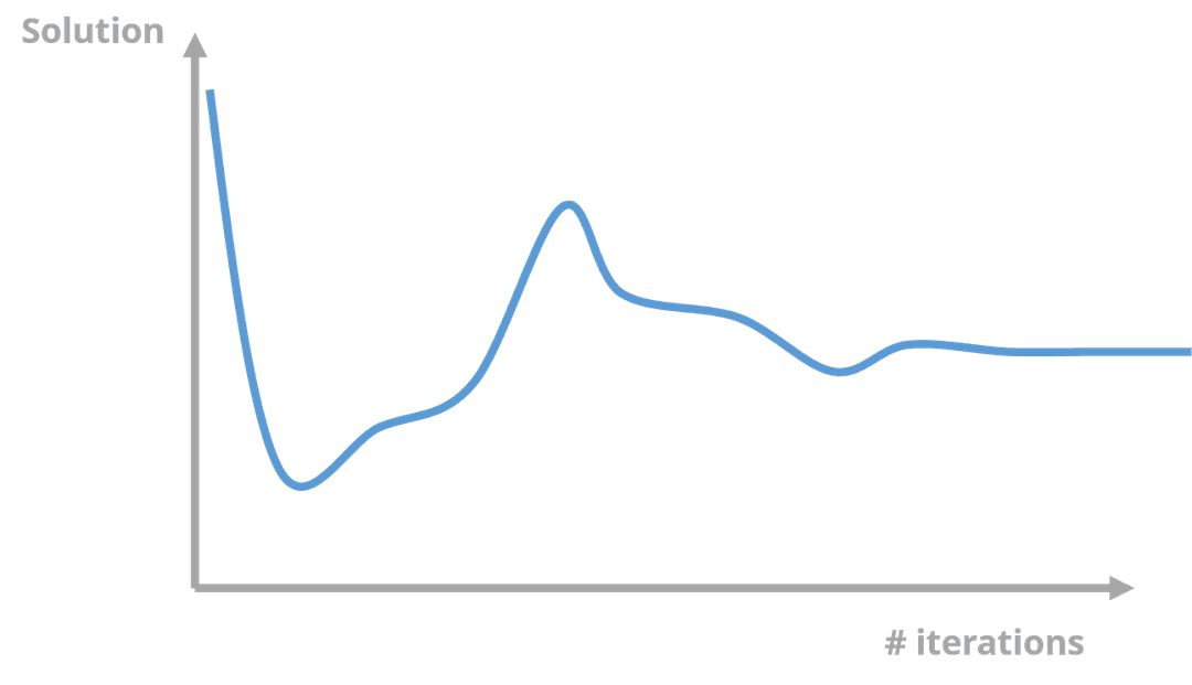
The iteration procedure works around all of the nodes until equilibrium is met for each time step. Of course, the easiest way to achieve an accurate solution is to keep iterating, but this is not computationally efficient. Instead, the user has to decide when the iteration error is acceptable. In the graph below, there are various points in the iteration count where the solution is relatively close or far away from the ultimate solution. Identifying this iteration error is not easy and depends on the purpose of each simulation.
Errors
When approximating solutions, it is important to understand the type and amount of error. The modelling stage is the first source of CFD software errors, which come in two forms. The first is the equations and simplifications that are chosen to be included in the model. This part of the equation can include many items that may or may not be relevant.
For example, if you are carrying out a CFD simulation of tides in the ocean, you have to include the gravitational force of the moon. However, this is not necessary when analysing the internal airflow in an automotive cooling system. Removing elements make the equations easier to solve, but this requires careful consideration to maintain accuracy.
The second source of error is the accuracy of the 3D CAD model, which may not include every detailed feature of the real object. Things like shut lines on car bodywork or rivet heads on an aircraft skin can completely change the boundary conditions and therefore the behaviour of the flow.
What can we do with our results?
Once we have a solution for the case, there is a huge amount of data available for processing. At each point in the mesh, we know the flow velocity and pressure which can be post-processed to generate more useful values. For example, to calculate the lift of an aircraft wing, the surface pressures on each node can be multiplied by the surface area that the node represents to calculate the force. Summing this for both the upper and lower surfaces of the wing determines the wing's lift.
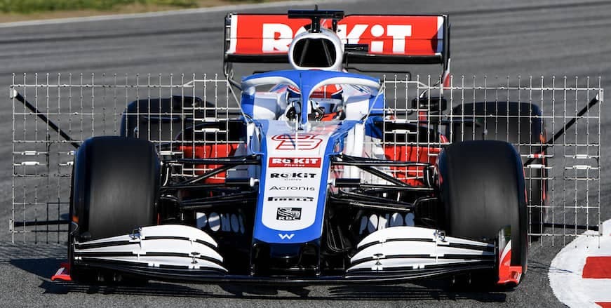
On a Formula 1 car, the aerodynamics are heavily dependent on managing vortex structures to generate downforce. Knowledge of the flow velocities u, v and w means these vortices can be easily visualised at x, y and z slices along the car. This is almost impossible to do in any other way.
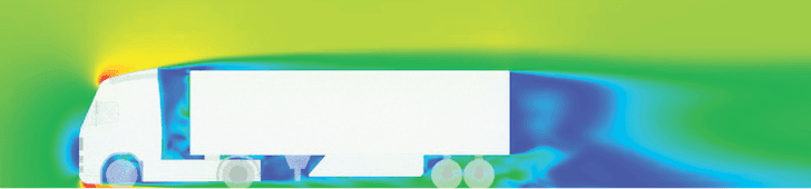
Formula 1 cars are a niche example, but this approach also works for other problems like drag on a heavy goods vehicle (HGV). Managing the surface friction and wake of a vehicle like this can save fuel and money and reduce carbon emissions.
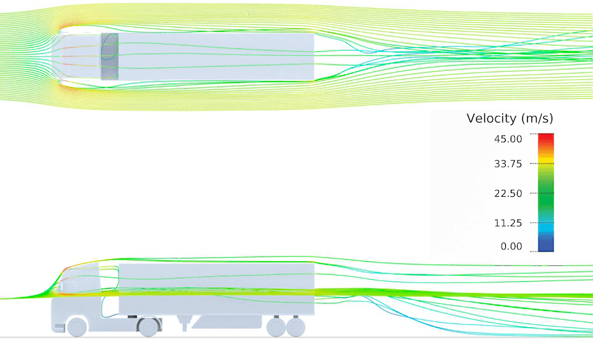
It is also possible to trace the path of an individual air particle to create a streamline, studying how it moves along the vehicle. This allows the user to see where the air impacting a surface is coming from.
Correlation
It's important to correlate the CFD results with physical tests in wind tunnels. Techniques like smoke visualisation, Particle Image Velocimetry (PIV) and kiel probe rakes are used to create flow visualisations to compare and validate CFD simulations.
Taking comparable slices through the flow field obtained using these physical test methods allow direct comparisons to be made to CFD cases. Any errors can be identified and solved. This may require changing solver steps, meshing or turbulence models until correlation improves. The confidence gained from the correlation procedure allows the CFD results to be used more widely.
The future of CFD
CFD users are already working with vast super computers with thousands of cores to solve their cases. Despite this, it is still very difficult to use CFD in a similar way to wind tunnels. A Formula 1 team using continuous motion in a wind tunnel can generate hundreds of downforce and drag numbers in a matter of hours. Doing the same in CFD, where each change in configuration is a new case, would take too long to solve, which is why wind tunnels are still used.
This is likely where the main advances in CFD will be made. Increases in computing power with cloud services, solver design and meshing software will make simulations faster and more accurate.
If mathematicians make progress with solving the Navier Stokes equations, this could also transfer into commercial CFD solvers. This could reduce the dependency on users when defining mesh and solver settings as well as starting conditions, iteration counts and turbulence models. Automating these settings in an intelligent and consistent way, such as with AirShaper, can help resolve some of the uncertainty and improve the reliability and accuracy of CFD simulations.
However, the rate of development of CFD solvers and computing power will boost the capabilities of CFD, allowing it to be used more frequently and for more complex applications. In fact, CFD is expected to become so accurate, that Formula 1 teams could ban wind tunnels from 2030.